ECON4004 Advanced Macroeconomics

Finally!!! The advanced level course taught in UM.

You can find the related materials in: ECON2005 Intermediate Macroeconomics

IS-LM model

Modern Macroeconomic model?

• Dynamic: The economic variable would change due to time, and is affected by policies.
• General Equilibrium: All economic agents in the market (households, firms, government, etc.) reach equilibrium at the same time and all markets are cleared (i.e. supply and demand are equal)

Dynamic General Equilibrium (DGE) is complicated.

---

Lecture 1 Macro Data

Two components:

1. Economic Growth: it determines the slope of the trend of GDP.
2. Business Cycle: it determines the fluctuations around the trend.

You used the Solow Model to study economic growth. You used IS-LM model (Keynesian) to study economic fluctuations.

Hamiltonian: Only need to apply, no need to prove, just like Largrangian Theory

4. Hamiltonian函数的经济含义：1. 代表了经济系统在某一时点的”总价值” 2. 包含了当期收益和未来价值的变化 3. $\lambda$表示状态变量的边际价值

In short, we will develop a modern macroeconomic model to study both growth and fluctuations.

It is also the purpose to study this course.

Modern Macroeconomic Model

It features dynamic general equilibrium (DGE) with microeconomic foundation.

Market Economy

Try to represent Market Economy using a simple graph.

Consumers ${\to }^{\text{output (good and services)}}$ Firm

Firms ${\to }^{\text{factor inputs (labor, capital)}}$ Consumers

In microeconomic foundation, consumers seek to maximize utility, and firms try to maximize profit. Consumers and firms interact in the labor market, the capital market, and the output market.

The road to study this course: Microeconomic Foundation → General Equilibrium → Dynamic, and this is the Modern Macro

We will study how the different markets affect each other.

Static General-Equilibrium Model

Firms maximize profit

Some notations:

• Profit: $\pi$

• Price: $p$

• Output: $Y$

• Labor: $L$

• Capital: $K$

• Wage: $w$

• Rental price of capital: $R$

• Technology: $A$

• Profit function of a firm: $\pi =pY-wL-rK$

• Production function: $Y=F(A,K,L)$

• Cobb-Douglas Production Function: $Y=A{K}^{\alpha }{L}^{1-\alpha }$

$\alpha \in [0,1]$ is the degree of capital intensity in production. In the real world data, $\alpha \in [0.3,0.5]$ (Western countries and China)

Recall the Profit function of a firm:

$\pi =pY-wL-rK$

Replace $Y$ by Cobb-Douglas Production Function

$\pi =PA{K}^{\alpha }{L}^{1-\alpha }-wL-rK$

FOC: $\frac{\delta \pi }{\delta K}=P\alpha A{K}^{\alpha -1}{L}^{1-\alpha }-r=0⟹\frac{r}{P}=\alpha A{\left(\frac{L}{K}\right)}^{1-\alpha }$ (The right hand side is the $MPK$)

→ this is the demand function for capital.

We could find that when $R$ increases, $K$ decreases, this is the law of demand, which reflects the concept of the microeconomic foundation

$\frac{\delta \pi }{\delta L}=P(1-\alpha )A{K}^{\alpha }{L}^{-\alpha }-w=0⟹\frac{w}{P}=(1-\alpha )A{\left(\frac{K}{L}\right)}^{\alpha }$

→ this is the demand function for labor.

Real wage = $MPL$ （Left hand side = Right hand side）

The capital demand curve would be like a decreasing convex c, this is the law of demand.

The lack of IS-LM model: it didn’t reflects the microeconomic foundation.

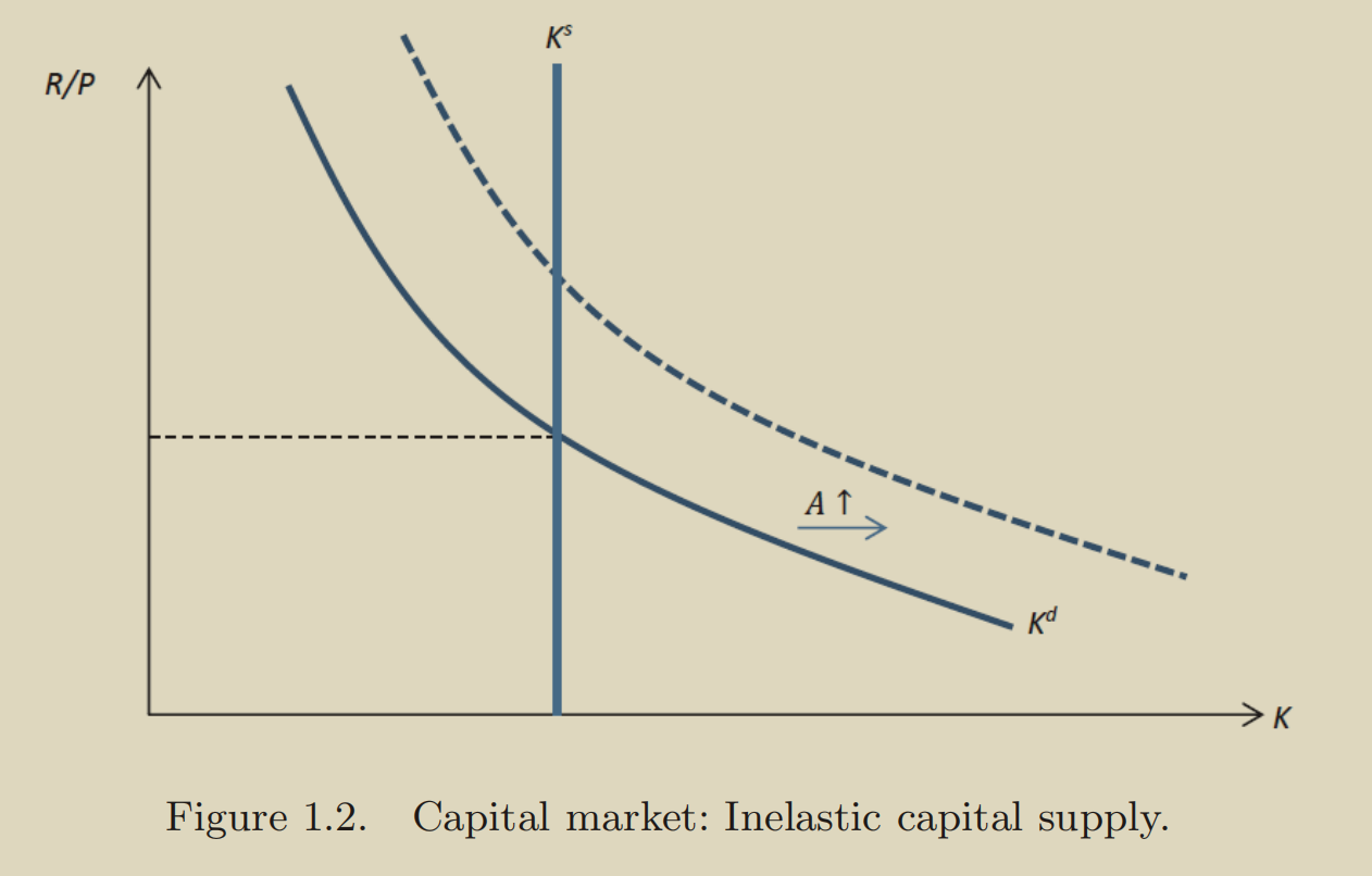
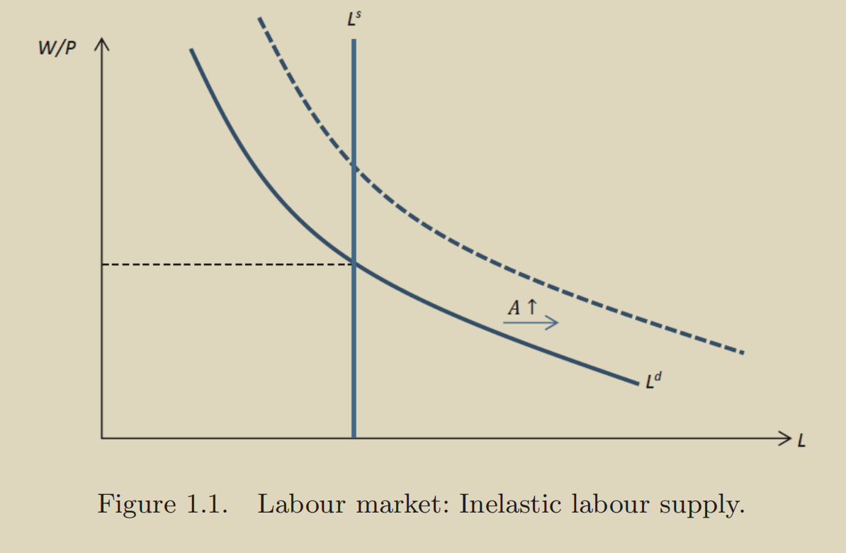
To draw the labor market and capital market is simple, we could derive the demand curve using the equations just mentioned before, to derive the supply curve, we simply make the labor supply be perfectly inelastic. (这里补一个图)

Question: What happens to the economy when $A$ goes up?

Answer: in both graph (capital and labor), the $L^d$ and $K^d$ both shift upwards. ($L^d$ and $K^d$)

In general,

• Labor Market: $\frac{w}{P}\uparrow ,\Delta L=0$
• Supply Market: $\frac{r}{P}\uparrow ,\Delta K=0$
• Output Market: $Y=A{K}^{\alpha }{L}^{1-\alpha }$

Since in the perfectly inelastic case, $K$ and $L$ don’t change, only $A\uparrow$, so $Y\uparrow$ also.

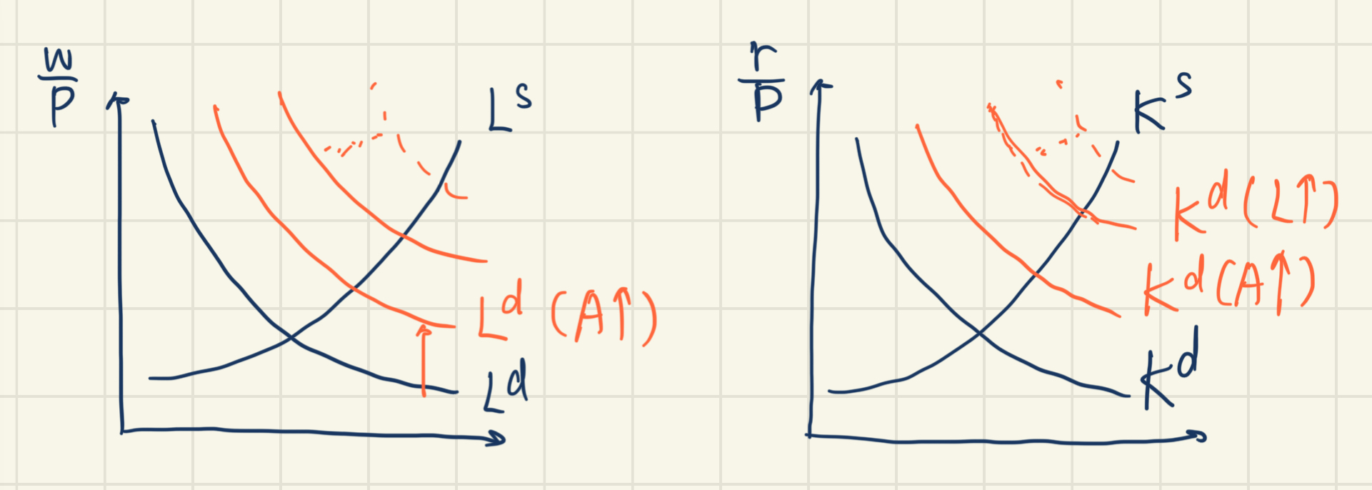
How about the elastic case?

Consider the elastic labor supply case:

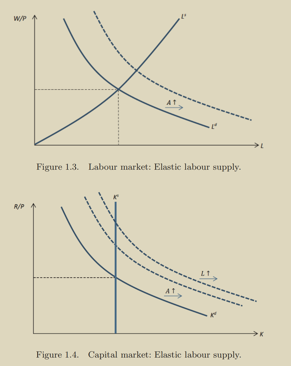
The key concept here is that, we recall the equation:

$\frac{r}{P}=\alpha A{\left(\frac{L}{K}\right)}^{1-\alpha }$

The result in the labor market is that the quantity of labor goes up, so that the change in the capital market should involves into an additional shift. ($A\uparrow$,$L\uparrow$)

In general,

• Labor Market: $\frac{w}{P}\uparrow ,L\uparrow$
• Supply Market: $\frac{r}{P}\uparrow ,\Delta K=0$
• Output Market: $Y=A{K}^{\alpha }{L}^{1-\alpha }$, $Y$ increases due to two reasons.

In conclusion, what happens in the labor market affects the capital market, this is a general-equilibrium effect.

What about both markets are elastic?

The intuition is that the process would be infinite, but finally the process would stop. (May because the productivity is limited)

• Labor Market: $\frac{w}{P}\uparrow ,L\uparrow$
• Supply Market: $\frac{r}{P}\uparrow ,K\uparrow$
• Output Market: $Y=A{K}^{\alpha }{L}^{1-\alpha }$, $Y$ increases due to three reasons.

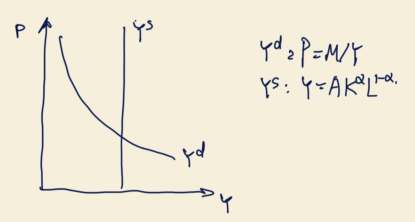
Lets try to draw the graph of output market is that since the $Y$ doesn’t matter with price, we first consider the real variables:

$\{L,K,Y,\frac{r}{P},\frac{w}{P}\}$

What determines

$\{P,w,r\}$

We need to introduce money to the model. The quantity theory of money is:

$$MV=PY$$

$M$ is the level of money supply, $V$ is the Velocity of Money.

For simplicity, we set $V=1,⟹M=PY⟹P=\frac{M}{Y}$

So, $P=\frac{M}{Y}$ is the demand function for $Y$,

$Y=A{K}^{\alpha }{L}^{1-\alpha }$ is the supply function for $Y$.

So the graph for output market would look like:

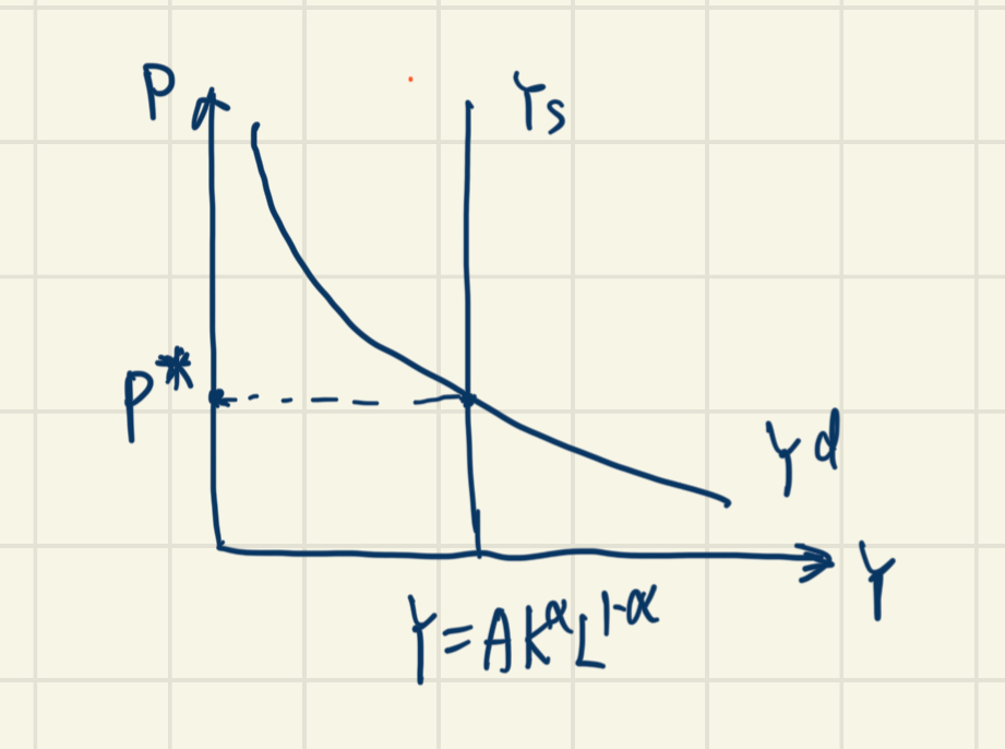
For example, when $A\uparrow$, the $Y^s$ shift to the right, $Y\uparrow$, $P\downarrow$

In this economy, the money is neutral.

This is different from the IS-LM model because they are focusing on different time horizon. This is called monetary neutrality, which captures the long-run effects of monetary policy.

We could determine the variables separately.

Key assumption: All prices are fully flexible. So money supply have no effect.

Exercise

Derive the equilibrium expression for $\{P,w,r\}$. Hint: $P(M,A,K,L)$, $W(M,L)$,$R(M,K)$

For $P$,

Since $MV=PY,V=1$, we could get:

$P=\frac{M}{Y}=\frac{M}{A{K}^{\alpha }{L}^{1-\alpha }}$

For $w$,

$\frac{w}{P}=(1-\alpha )A{\left(\frac{K}{L}\right)}^{\alpha }$

We substitute $P$:

$w=\frac{M}{A{K}^{\alpha }{L}^{1-\alpha }}(1-\alpha )A{\left(\frac{K}{L}\right)}^{\alpha }=\frac{(1-\alpha )M}{L}$

Similarly, we could get $r=\frac{\alpha M}{K}$

Classical Dichotomy

Quick Review

We used the labour market, the capital market and the production function to determine $\left\{\frac{w}{p},\frac{r}{p},L,K,Y\right\}$.

They are the real variables.

How about the nominal variables? $\{w,r,R\}$?

We use the quantity theory of money: $MV=PY$

The reason we could make it is that money has no effect on the real economy. This is called monetary neutrality. We have monetary neutrality in this economy because all the prices are fully flexible. So, money only affects the nominal variables.

For example, we derive $w$:

$$\begin{array}{rl}\frac{w}{p}& =MPL=(1-\alpha ){\left(\frac{K}{L}\right)}^{\alpha }\\ w& =(1-\alpha ){\left(\frac{K}{L}\right)}^{\alpha }p\\ w& =(1-\alpha ){\left(\frac{K}{L}\right)}^{\alpha }\frac{M}{A{K}^{\alpha }{L}^{1-\alpha }}\\ w& =\frac{(1-\alpha )M}{L}\end{array}$$

Summary

$M\uparrow ,⟹P\uparrow ,w\uparrow ,r\uparrow$ (Nominal variable)

However, $M$ has no effect on the real variables. Thus we have monetary neutrality due to flexible prices.

Chapter 2 The Neoclassical Growth Model

Now we want to define the supply side. We pick $Y$ as the numeraire.($P=1$)（计量标准）(Recall that the firms try to maximize the profit)

And Households supply labour inelastically: $L^s=\bar{L}$, so that $L^s$ is a parameter.

We allow for an elastic supply curve of capital. Households maximize utility to determine consumption and saving. Saving affect capital accumulation via capital investment.

Households

Households maximize utility. $U(C)=lnC$

The reason we choose this function is because it has some nice properties:

1. Diminishing Marginal Utility (It is increasing in a decreasing way), that’s also the reason why we don’t use a simple linear function.
2. If $li{m}_{C\to 0}lnC=-\infty$
3. $\frac{\delta U}{\delta C}=\frac{\delta lnC}{deltaC}=\frac{1}{C}$

We care about the lifetime utility function, then it is obvious that we could derive the utility function:

$U={\sum }_{t=0}^T{u}_t={\sum }_{t=0}^{T}ln{C}_t$

People discount the future utility. We then introduce the discount rate $\rho$. (recall Game Theory)

$$U=U_0+\frac{U_1}{1+\rho }+\frac{U_2}{(1+\rho {)}^2}+\cdots +\frac{U_T}{(1+\rho {)}^T}=\sum _{t=0}^T{U}_t/(1+\rho {)}^t$$

So the lifetime utility is:

$$U=\sum _{t=0}^T\frac{U_t}{(1+\rho {)}^t}$$

And we approximate $T$ by $\infty$

$$U=\sum _{t=0}^{\infty }\frac{U_t}{(1+\rho {)}^t}$$

This is a discrete-time model. However, time is a continuous variable, we want to convert the discrete-time utility function into a continuous-time utility function by replacing the summation sign with an integral sign.

$$U={\int }_0^{\infty }{U}_{t}dt\text{(without discounting)}$$ $$U={\int }_0^{\infty }{e}^{-\rho t}{U}_{t}dt\text{(with discounting)}$$

Thus the households’ objective is

$$Ma{x}_{C_t}U=\sum _{t=0}^{\infty }\frac{U_t}{(1+\rho {)}^t}$$

Without the constraint, the best way for us is to take $C_t\to \infty$ in every period. In reality, the households faces budget constraint

Hamiltonian

Multiplier ${\lambda }_t$ is for the asset-accumulation equation.

$$\text{Income}=\text{Consumption}+\text{Saving}$$

The word “Saving” here is flow, not stock (saving in your bank).

$$\text{Income}=WL+RK$$

For consumers, and we denote consumption by $C$, and saving by $I$(Capital Investment), because we assume that capital is the only productive asset in the economy. Investment today becomes capital in the future.

记住大 $C$ 一般代表的就是 consumption

So the question becomes: how we could balance the investment in the certain period? Then we introduce the hamiltonian:

We define: $\dot{K}=\frac{\delta K}{\delta t}=\text{Capital Accumulation}$

So it’s trivial that $\dot{K}=RK+WL-C$

Recall that our objective is the Households’ optimization problem

$$Ma{x}_{C_t}U=\sum _{t=0}^{\infty }\frac{U_t}{(1+\rho {)}^t}$$

We will use a mathematical tool, known as the Hamiltonian, to solve this dynamic optimization problem.

In general, we want to compute that:

$$Ma{x}_{C_t}U=\sum _{t=0}^{\infty }\frac{U_t}{(1+\rho {)}^t}\text{subject to }\dot{K}=I=WL+RK-C$$ $$H_t=ln{C}_t+{\lambda }_t(R_t{K}_t+W_{t}L-C_t)$$

Then we find the first-order condition:

$$\frac{\delta H}{\delta C}=\frac{1}{C}-\lambda =0⟹\lambda =\frac{1}{C}=M{U}_0+C$$ $$\frac{\delta H}{\delta K_t}={\lambda }_t{R}_t=\rho \lambda -\dot{\lambda }⟹\frac{-\dot{\lambda }}{\lambda }=R-\rho$$

• $\lambda$ is a multiplier (or a costate variable)
• $K$ is a predetermined variable (or a state variable)
• $C$ is a jump variable

Then we try to manipulate FOCs:

$$\lambda =\frac{1}{C}=C^{-1}⟹ln\lambda =ln{C}^{-1}=-lnC$$ $$\frac{\delta ln\lambda }{\delta t}=\frac{1}{\lambda }\frac{\delta \lambda }{\delta t}=\frac{\dot{\lambda }}{\lambda }=\text{growth rate of}\lambda$$

Similarly,

$$\frac{\delta -lnC}{\delta t}=\frac{\dot{C}}{C}$$

That means:

$$\frac{\dot{\lambda }}{\lambda }=\frac{-\dot{C}}{C}$$

Recall the equation:

$$\frac{\delta H}{\delta K_t}={\lambda }_t{R}_t=\rho \lambda -\dot{\lambda }⟹\frac{-\dot{\lambda }}{\lambda }=R-\rho$$

We get:

$$\frac{-\dot{\lambda }}{\lambda }=\frac{\dot{C}}{C}=R-\rho$$

This is the optimal path of consumption chosen by the household.

We could also write it as: $\frac{{\dot{C}}_t}{C_t}=R_t-\rho$

This is the optimal consumption growth rate.

• If $R_t>\rho$, then $\frac{\dot{C}}{C}>0$

Intuitively speaking, if the return to capital ($R$) is high, then the optimal behavior is to save more and consume less today. So, the household’s consumption is rising overtime.

We save for future consumption

Firms

To find the equilibrium, we need both the decisions from firms and Households. For households, we need to maximize the profit. And typically we use the Cobb-Douglas Production Function in practice:

$$Y=A{L}^{\alpha }{K}^{\beta }$$

For a firm, its profit = revenue ($Y$) minus its cost, which is $wL+rK$, so

$$\pi =Y-rK-wL$$

Take the first order condition:

$$\frac{\partial {\Pi }_t}{\partial K_t}=\frac{\partial Y_t}{\partial K_t}-r_t=\underset{MPK}{\underbrace{\alpha A{K}_t^{\alpha -1}{L}_t^{1-\alpha }}}-R_t=0,$$ $$\frac{\partial {\Pi }_t}{\partial L_t}=\frac{\partial Y_t}{\partial L_t}-W_t=\underset{MPL}{\underbrace{(1-\alpha )A{K}_t^{\alpha }{L}_t^{-\alpha }}}-W_t=0.$$

The important thing is to notice the $MPK$ and $MPL$.

The Steady State Equilibrium

Recall from the households, we already find that in steady state,

$\frac{{\dot{C}}_t}{C_t}=r_t-\rho$. In the $MPK$ function, we also have a function with $r$

So

$$\frac{{\dot{C}}_t}{C_t}=\underset{MPK}{\underbrace{\alpha A{K}_t^{\alpha -1}{L}_t^{1-\alpha }}}-\rho$$

Finally we could get the $\dot{K}$, where

$$\dot{K}=A{K}^{\alpha }{L}^{1-\alpha }-C$$

Recall that we have fixed the $L$, so from the equations, the change in $C$ and $K$ are those who determine the behavior of the economy.

At the steady state ($\dot{C}=0$)

$$\begin{array}{r}0=\alpha A{K}^{\alpha -1}{L}^{1-\alpha }-\rho \\ K^{\ast }={\frac{\alpha A}{\rho }}^{1/1-\alpha }L\end{array}$$

We could put it back into the production function, then we get:

$$Y^{\ast }=A{\frac{\alpha A}{\rho }}^{1/1-\alpha }L{L}^{1-\alpha }={\left(\frac{\alpha A}{\rho }\right)}^{\frac{\alpha }{1-\alpha }}AL$$

At the steady state $\dot{K}=0$,

$$C^{\ast }={\left(\frac{\alpha A}{\rho }\right)}^{\frac{\alpha }{1-\alpha }}AL$$

that $C=Y$. In this special case, we assume no depreciation rate ($\delta =0$), so that $I^{\ast }=Y^{\ast }-C^{\ast }=0$

Chapter 3 Dynamics in the Neoclassical Growth Model

Recall that the Steady State means that we capture the long-run effect, but it’s not enough.

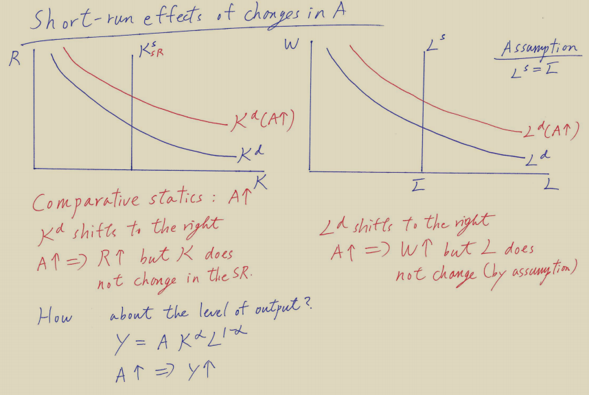
In this chapter, we try to study the short-run effects in the change in technology $A$.

• Why the short-run supply curve of capital is vertical?

Because at the moment when $A$ changes, the level of capital in the economy is predetermined and cannot change immediately.

Also, notice that we assume a perfectly inelastic labour supply, so the labour supply curve is also vertical.

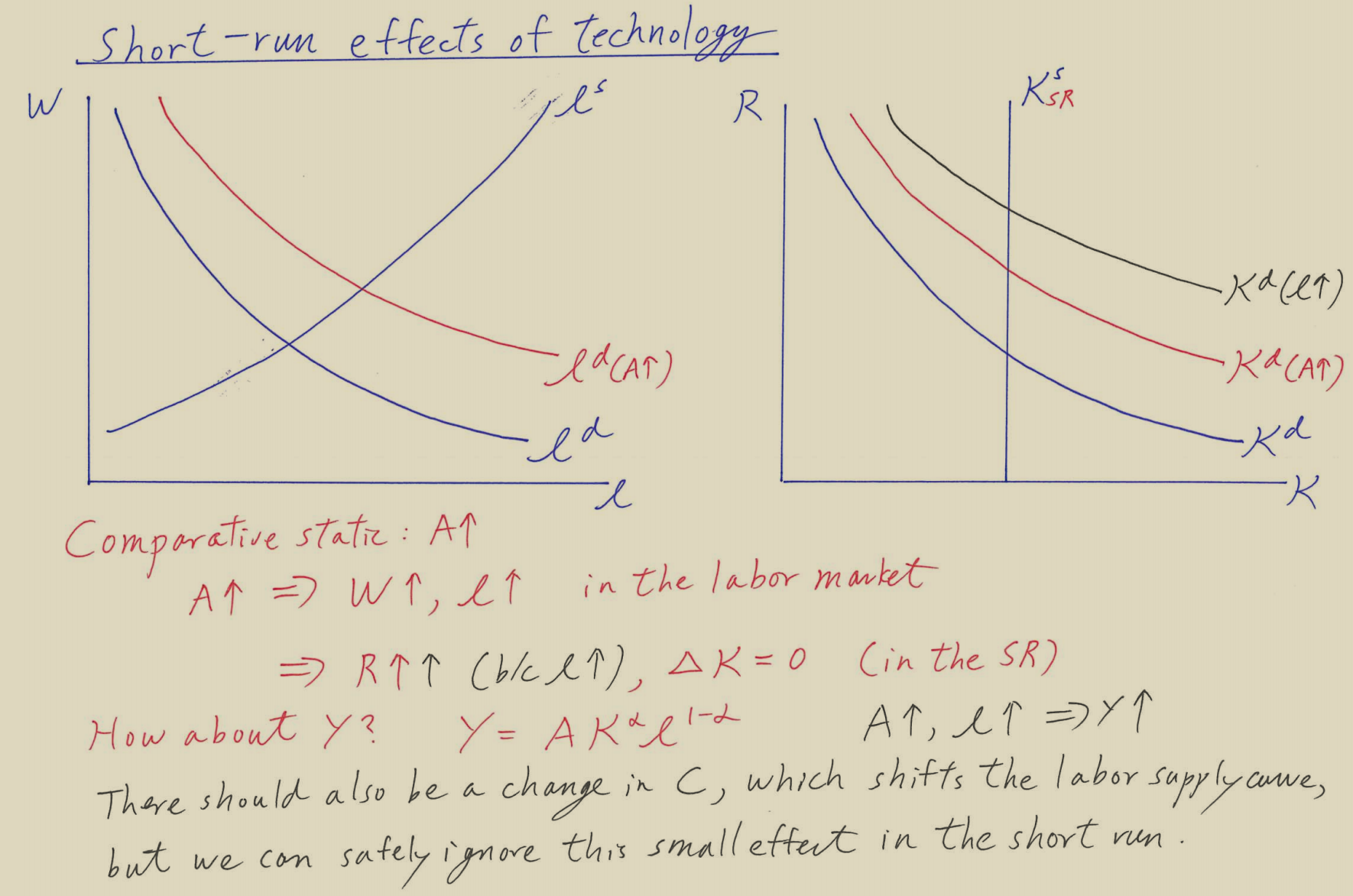
Short-Run Effects of Technology

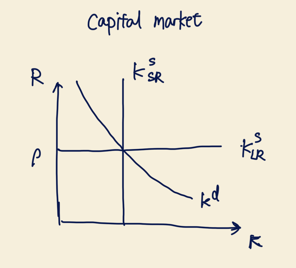
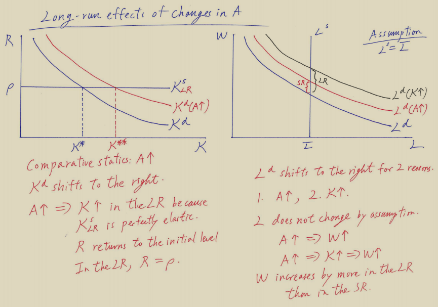
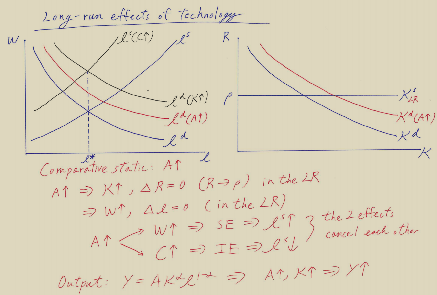
Long-Run Effects of Technology

The long-run capital supply curve

Recall that Steady state means long-run equilibrium.

All variables remain constant:

$$\dot{C}=0⟹\frac{\dot{C}}{C}=0=R-\rho ⟹R=\rho$$

So that in the long-run, the capital supply is a horizontal line, $R=\rho$. The intuition is that $\rho$ is a constant, and it won’t change. We are looking at the case when it is long-run. So we make sure $r=\rho$, which is a horizontal line.

• $K_{LR}^s:R=\rho$, it will be a horizontal line (perfectly elastic)
• $K^d:R=MPK=\alpha A{\left(\frac{L}{K}\right)}^{1-\alpha }$

In the short-run, the supply would be perfectly inelastic, because $K$ is predetermined variable

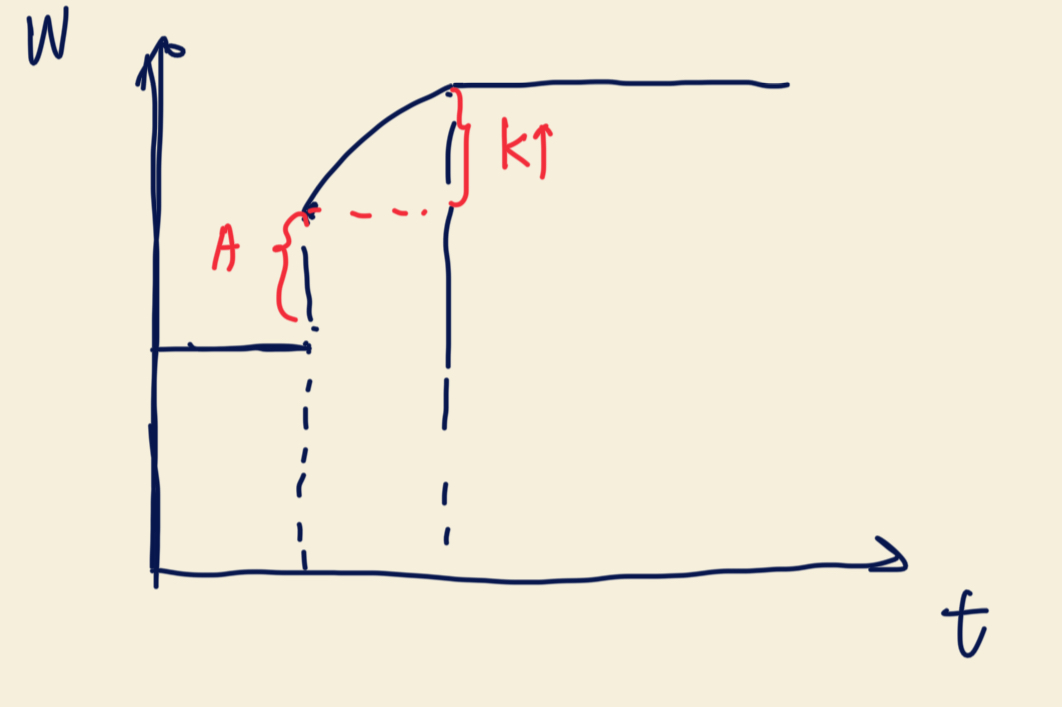
What happens to output?

$Y=A{K}^{\alpha }{L}^{1-\alpha }$

$Y$ increase for 2 reasons.

Exercise

Question: Derive the steady-state level of capital. Show that $K^{\ast }(A(+))$

Hint: Combine $K^d$ and $K^S$

Comparative static: $A\uparrow$.

In the SR, $A\uparrow ⟹R\uparrow$ and $K$ remains at $K^{\ast }$ at this moment. Overtime, $K$ gradually increases, and $R$ gradually decreases.

In the LR, $K\to K^{\ast \ast }$ and $R$ return to $\rho$.

In the SR, $r>\rho ⟹\frac{\dot{C}}{C}>0$

The household reduces current consumption and increases saving, so that capital investment goes up.

---

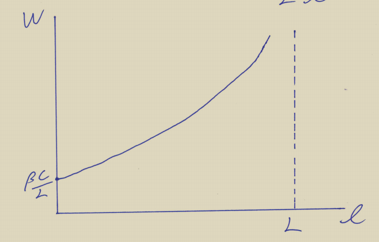
The time path

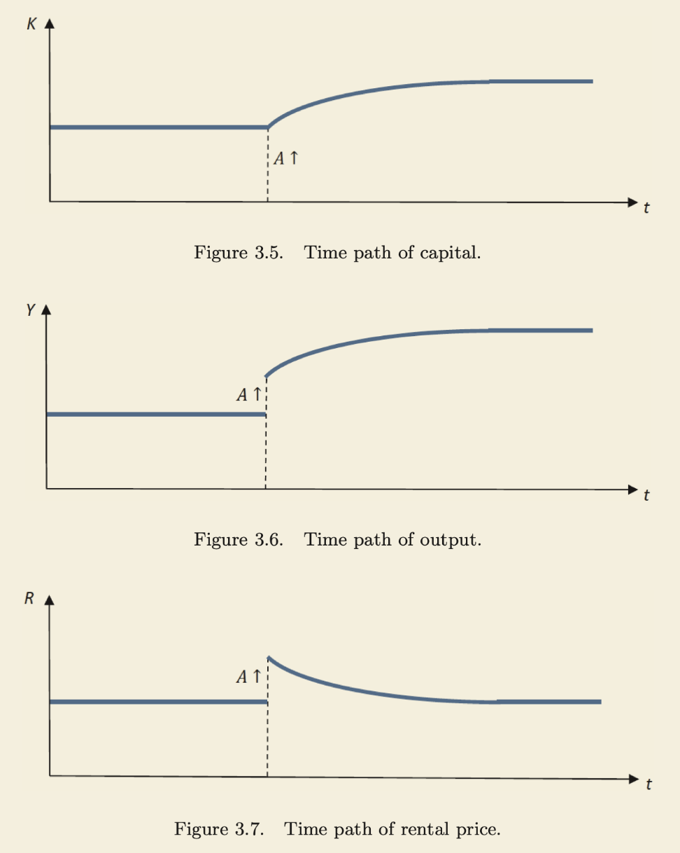
Note that the shape of $K$ is concavely decrease.

In the labor market, recall that $L^d:w=MPL=(1-\alpha )A{\left(\frac{K}{L}\right)}^{\alpha }$

Real Business Cycles model, Kyland and Prescott won a Nobel prize for developing the RBC model

Exercise

$ma{x}_{C_t}U={\sum }_{t=0}\frac{ln{C}_t}{(1+\rho {)}^t}$ s.t. $\dot{K}=I-\delta K=WL+RK-C-\delta K$

$\delta$ is the capital depreciation rate.

Use Hamiltonian to solve it:

$$H=lnC+\lambda \dot{K}$$

• $\frac{\delta H}{\delta C}=\frac{1}{C}-\lambda =0⟹\lambda =\frac{1}{C}=M{U}_0+C$
• $\frac{\delta H}{\delta K}=\lambda (R-\delta )=\rho \lambda -\dot{\lambda }⟹-\frac{\dot{\lambda }}{\lambda }=R-\delta -\rho$

IMPORTANT: We should take the derivative for $\lambda$ and $\frac{1}{C}$, and then we could get $\frac{\dot{C}}{C}=R-\delta -\rho$

Optimal Consumption Path

If the net return to capital is high relative to the household subjective discount rate (how patient it is), then the household wants to invest more in capital. As a result, consumption is lower today and rising overtime.

Chapter 4 The Neoclassical Growth Model with Elastic Labour Supply

What’s the disadvantages in Chapter 3 is that We made a very ‘hard’ assumption, that the labour is perfectly inelastic. In this chapter, we try to generalize it.

Households

We consider a background info.

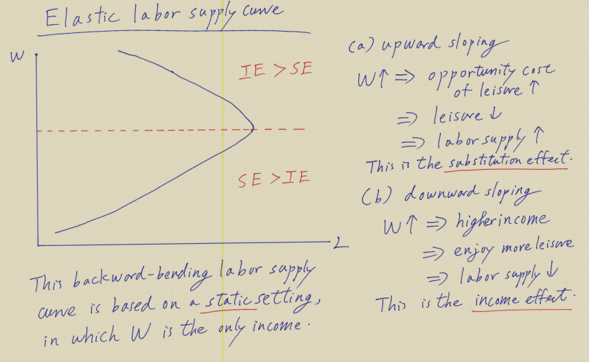
The supply of labour is basically determined by two aspects: the Substitution Effect and the Income Effect.

In this setting, we introduce a new variable, $l$ as “Employment”.

Since the total labor is $L$, the leisure the households enjoy now is $L-l$. and we have also introduce $\beta$, which is the leisure preference parameter. The higher the $\beta$, the more the households would like to leisure.

Recall that the households would like to maximize their utility:

$$Ma{x}_{C_t,l_t}U=\sum _{t=0}\frac{u_t}{(1+\rho {)}^t}=\sum _{t=0}\frac{\ln C_t+\beta \ln (L-l_t)}{(1+\rho {)}^t}$$

s.t. $\dot{K_t}=I_t=r_t{K}_t+w_t\underset{\text{What’s different}}{\underbrace{l_t}}-C_t$

Hamiltonian

We can do the Hamiltonian again and then get:

$$\begin{array}{rl}\frac{\delta H}{\delta C}& =\frac{1}{C}-\lambda =0⟹\lambda =\frac{1}{C}\\ \frac{\delta H}{\delta K_t}& ={\lambda }_t{R}_t=\rho \lambda -\dot{\lambda }⟹\frac{-\dot{\lambda }}{\lambda }=r-\rho \end{array}$$

These two terms are the same, however, as for the labour,

$$\frac{\partial H}{\partial l}=-\frac{\beta }{L-l}+\lambda w=0$$

We could then derive the labour supply curve as:

$$l^s=L-\frac{\beta C}{w}$$

Some intuitions behind it:

1. When $\beta =0$, then $l=L$
2. When $\beta >0$, then $l>0$. It shows the properties of $\beta$.

The wage $w$ shows the Substitution Effect. Because from the Hamiltonian, we see that $\lambda w=\frac{\beta }{L-l}$. It is the marginal utility of leisure. We fix $\lambda$, then when $w$ increases, the Opportunity Cost of leisure increases, and then the household would like to supply more labour. And this is the Substitution Effect.

We could see that $l$ is a function of $C$ and $w$. The formal one is the Income Effect because it is a function of current and future income. So it could capture the entire Income Effect.

We first fix $w$, from $\frac{\delta H}{\delta C}=\frac{1}{C}-\lambda =0⟹\lambda =\frac{1}{C}$, when $C$ increases, $\lambda$ decreases. Recall the function: $\lambda w=\frac{\beta }{L-l}$, since $\lambda$ decreases, what’s most important is that $\frac{\beta }{L-l}$ is directly the Marginal Utility of Leisure (Same as how we derive $MPK$, $MPL$, etc.) So $M{P}_{\text{Leisure}}$ also decreases.

Firms

The only things that changes in the function is $L$ to $l$.

That the Cobb-Douglas Production Function becomes:

$$Y=A{K}^{\alpha }{l}^{1-\alpha }$$

So does the profit function $\Pi$.

Short-Run Effect on Technology

The labour supply curve now is given by:

$$w=\frac{\beta C}{L-l}$$

which is upward-sloping.

Fiscal Policy

The Midterm Exam would cover from Ch1-Ch7

• Do the Math
• Do the Graph

Economic Growth

• Highest GDP per capita > \100k$ (PPP adjusted)

Examples: Macau (\130k$),Singapore($$148k$)Luxembourg($$ 151k$)

• Lowest GDP per capita: ~ \ 1k$

Examples: South Sudan: (\760$),CentralAfricanRepublic($$1300$)

Fact 1: Income Differences across countries are extremely large and can be over 100 times between the richest and poorest economies in the world.

Simple Example

Country	1820	2020
A	\1000$with$g=1%$	\7000$
B	\1000$with$g=2%$	\52000$

Fact 2: A small growth differential accumulated over a very long period of time can lead to large income differences.

$$GDP=\text{output of an economy}$$

Aggregate Production Function

It has combination of: $Y=F(A,K,L,N,H\dots )$

Growth in output $Y$ must come from growth in the inputs.

Some notations:

• $Y$: output

Proximate Causes:

• $A$: technology - technology progress
• $K$: capital - capital accumulation
• $L$: labor - population growth
• $N$: natural resources -discovery
• $H$: human capital - education

Those factors would lead to economic growth in $Y$.

Fundamental Causes

• Institutions eg. property rights
• Geography eg. international trade
• Culture: eg. saving/eduction
• Luck eg. natural resources

Solow Model

See the notes above.

Midterm: Neoclassical model and application

---

Some Questions for ECON4004 (Todo)

• Is Capital = Saving = Investment in Neoclassical Growth Model?

Sample Exam Question Self-Answer

Question: Discuss the Neoclassical growth model with elastic labour supply and apply it to demonstrate the short-run and long-run effects of an increase in the government-spending ratio (financed by a lump-sum tax) on the economy. How would your results change if labour supply were perfectly inelastic?

We define that $\gamma$ as the government-spending ratio.

Final Review

• Chapter 9: Solow Model
• Chapter 10-12: Ramsey Model
• Chapter 13: Romer Model