Static General-Equilibrium Model

Macro

Introduction

Before diving into the concepts, we have to first keep some things in mind: Firms always try to maximize profit, while households try to maximize their utility. In other words, if we could find the equilibrium using these two sides, we could get the answers to a lot of problems.

And clearly, we will solve the firm side, and the households side.

Some notations:

• Profit: $\pi$

• Price: $p$

• Output: $Y$

• Labor: $L$

• Capital: $K$

• Wage: $w$

• Rental price of capital: $R$

• Technology: $A$

• Profit function of a firm: $\pi =pY-wL-rK$

• Production function: $Y=F(A,K,L)$

• Cobb-Douglas Production Function: $Y=A{K}^{\alpha }{L}^{1-\alpha }$

Model

Firms

Recall that we use the Cobb-Douglas Production Function, which is useful. We first assume that the households supply inelastic labour and capital, which means $L^s=\bar{L}$, and $K^s=\bar{K}$. And we could consider them as exogenous parameters.

After production, the firms get the output $Y$:

$$Y=A{K}^{\alpha }{L}^{1-\alpha }$$

$\alpha \in [0,1]$ is the degree of capital intensity in production. In the real world data, $\alpha \in [0.3,0.5]$ (Western countries and China)

The Profit function of a firm:

$$\pi =pY-wL-rK$$

It’s just like $\pi =TR-TC$

Replace $Y$ by Cobb-Douglas Production Function:

$\pi =pA{K}^{\alpha }{L}^{1-\alpha }-wL-rK$

FOC: $\frac{\delta \pi }{\delta K}=p\alpha A{K}^{\alpha -1}{L}^{1-\alpha }-r=0⟹\frac{r}{P}=\alpha A{\left(\frac{L}{K}\right)}^{1-\alpha }$ (The right hand side is the $MPK$)

→ this is the demand function for capital. And the $\frac{r}{P}$ is the real rental price.

We could find that when $R$ increases, $K$ decreases, this is the law of demand, which reflects the concept of the microeconomic foundation

$\frac{\delta \pi }{\delta L}=P(1-\alpha )A{K}^{\alpha }{L}^{-\alpha }-w=0⟹\frac{w}{P}=(1-\alpha )A{\left(\frac{K}{L}\right)}^{\alpha }$

→ this is the demand function for labor. We could derive that:

$$L^d={\left[\frac{(1-\alpha )A}{w/p}\right]}^{1-\alpha }K$$

Real wage = $MPL$ （Left hand side = Right hand side）

The capital demand curve would be like a decreasing convex c, this is the law of demand.

The lack of IS-LM model: it didn’t reflects the microeconomic foundation.

To draw the labor market and capital market is simple, we could derive the demand curve using the equations just mentioned before, to derive the supply curve, we simply make the labor supply be perfectly inelastic. (这里补一个图)

Question: What happens to the economy when $A$ goes up?

Answer: in both graph (capital and labor), the $L^d$ and $K^d$ both shift upwards. ($L^d$ and $K^d$)

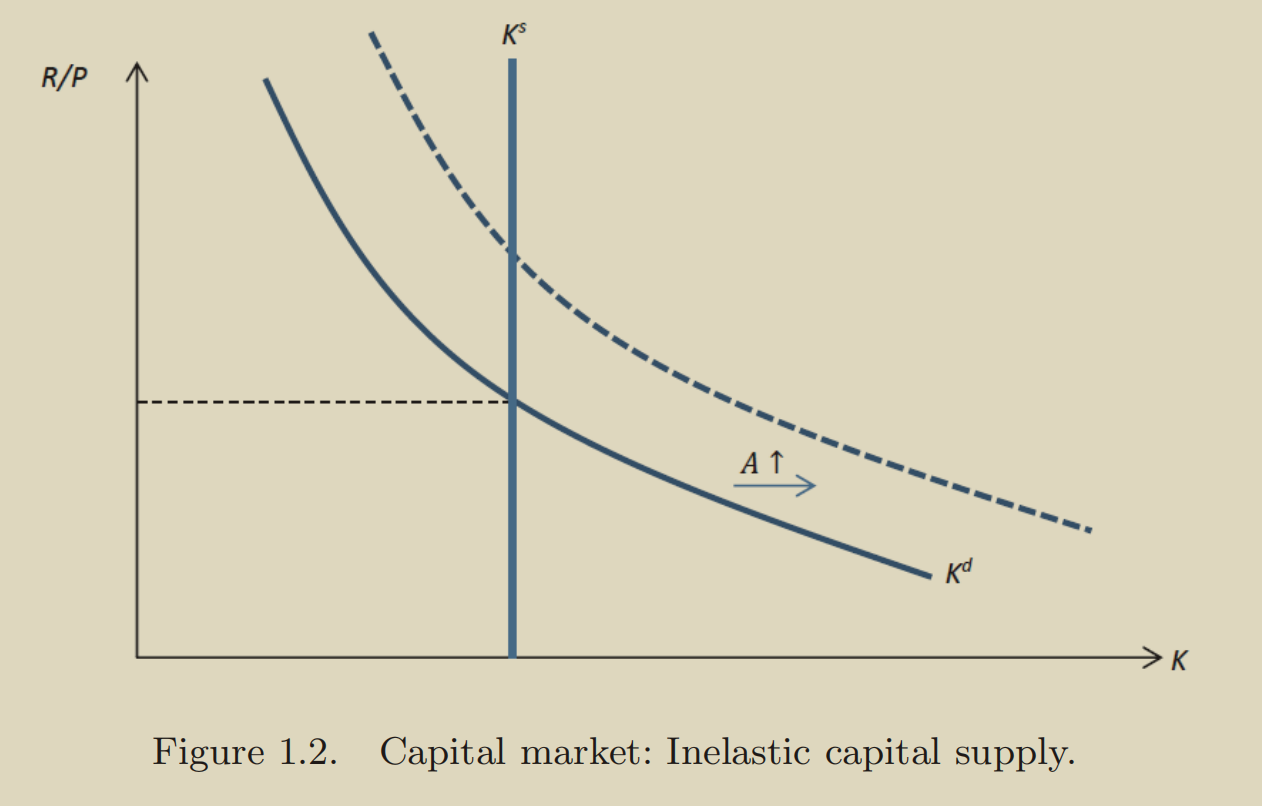
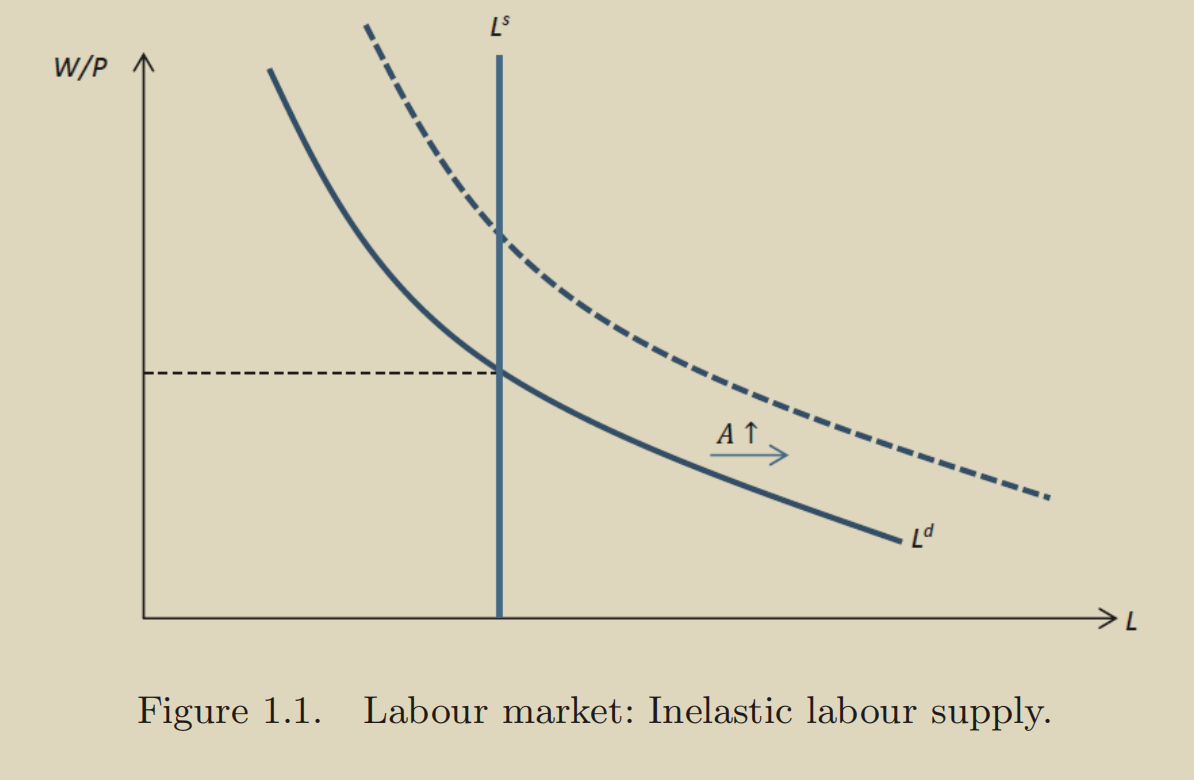
In general,

• Labor Market: $\frac{w}{P}\uparrow ,\Delta L=0$
• Supply Market: $\frac{r}{P}\uparrow ,\Delta K=0$
• Output Market: $Y=A{K}^{\alpha }{L}^{1-\alpha }$

Since in the perfectly inelastic case, $K$ and $L$ don’t change, only $A\uparrow$, so $Y\uparrow$ also. Because we assume both $K^s$ and $L^s$ are inelastic.

How about the elastic case?

Consider the elastic labour supply case:

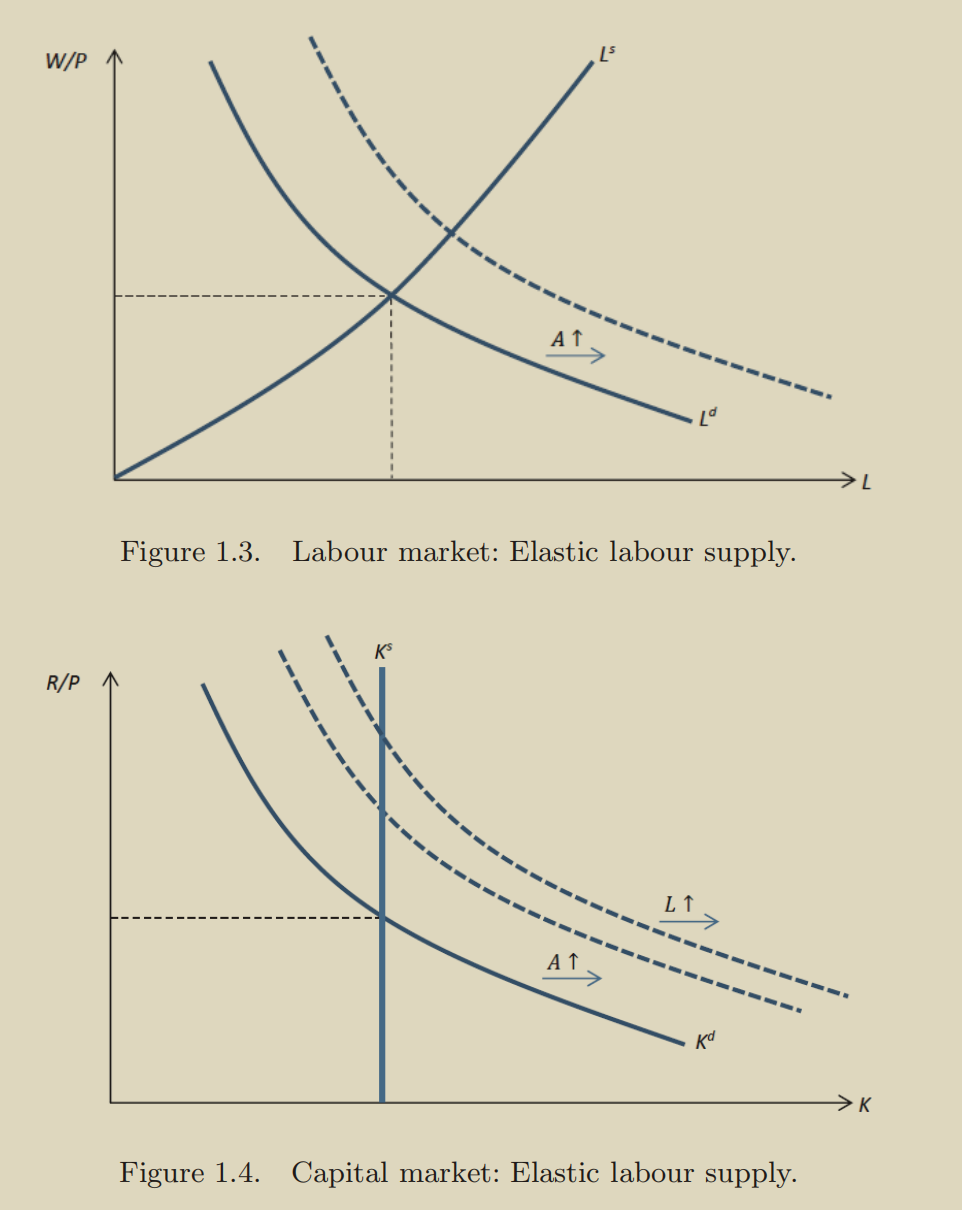
The key concept here is that, we recall the equation:

$\frac{r}{P}=\alpha A{\left(\frac{L}{K}\right)}^{1-\alpha }$

The result in the labor market is that the quantity of labor goes up, so that the change in the capital market should involves into an additional shift. ($A\uparrow$,$L\uparrow$)

In general,

• Labor Market: $\frac{w}{P}\uparrow ,L\uparrow$
• Supply Market: $\frac{r}{P}\uparrow ,\Delta K=0$
• Output Market: $Y=A{K}^{\alpha }{L}^{1-\alpha }$, $Y$ increases due to two reasons.

In conclusion, what happens in the labor market affects the capital market, this is a general-equilibrium effect.

What about both markets are elastic?

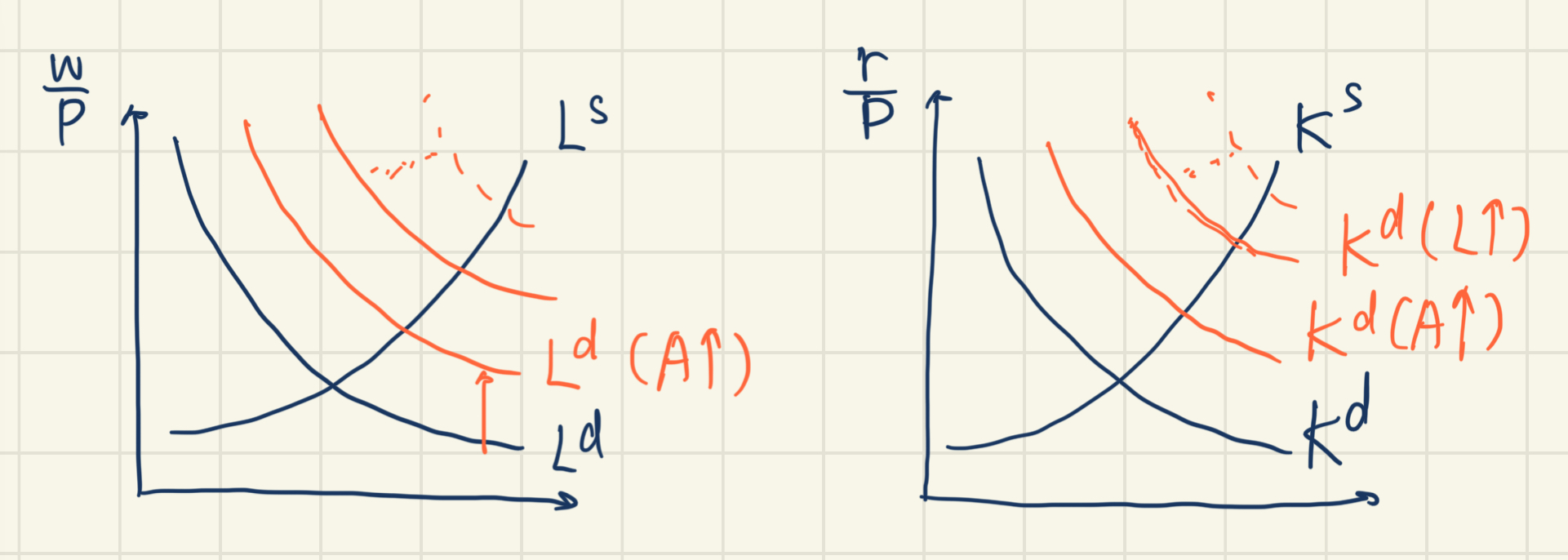
The intuition is that the process would be infinite, but finally the process would stop. (May because the productivity is limited)

• Labor Market: $\frac{w}{P}\uparrow ,L\uparrow$
• Supply Market: $\frac{r}{P}\uparrow ,K\uparrow$
• Output Market: $Y=A{K}^{\alpha }{L}^{1-\alpha }$, $Y$ increases due to three reasons.

Lets try to draw the graph of output market is that since the $Y$ doesn’t matter with price, we first consider the real variables:

$\{L,K,Y,\frac{r}{P},\frac{w}{P}\}$

What determines the nominal variables?

$\{P,w,r\}$

We need to introduce money to the model. The quantity theory of money is: (See Neutrality of Money)

$$MV=PY$$

$M$ is the level of money supply, $V$ is the Velocity of Money.

For simplicity, we set $V=1,⟹M=PY⟹P=\frac{M}{Y}$

So, $P=\frac{M}{Y}$ is the demand function for $Y$,

$Y=A{K}^{\alpha }{L}^{1-\alpha }$ is the supply function for $Y$. Since we have both supply and demand function, we are able to combine them and get the equilibrium.

So the graph for output market would look like:

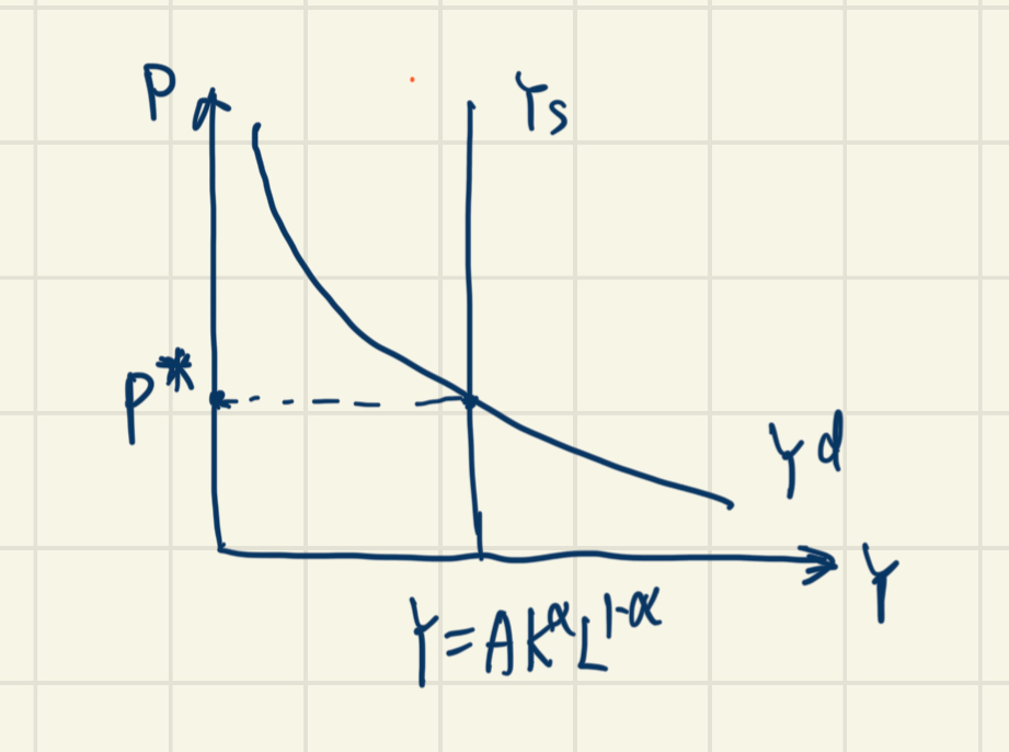
Supply Function

For example, when $A\uparrow$, the $Y^s$ shift to the right, $Y\uparrow$, $P\downarrow$

In this economy, the money is neutral. That is to say, the changes in the money supply do not affect real economic variables (such as output, employment, or real wages) in the long run.

This is different from the IS-LM model because they are focusing on different time horizon. This is called monetary neutrality, which captures the long-run effects of monetary policy.

We could determine the variables separately.

Demand Function

What happens when $M\uparrow$?

Recall that $P=\frac{M}{Y}$, so that when $M\uparrow$, $Y^d$ shifts to the right. So that $P\uparrow$, $\Delta Y=0$. This is called the monetary neutrality, which captures the long-run effects of monetary policy.

Key assumption: All prices are fully flexible. So money supply have no effect.