Nonparametric Method

metrics EC484_Econometrics_Analysis

Motivation

In econometrics, we often want to understand the relationship between two variables, say $Y$ and $X$. While parametric methods like linear regression assume a specific functional form for this relationship, nonparametric methods allow us to estimate it without such assumptions. This is particularly useful when the true relationship is complex or unknown. The idea is that we don’t assume the form of the relationship between $Y$ and $X$, but instead let the data speak for itself.

Basic Idea

Consider an i.i.d. sample $\{X_i{\}}_{i=1}^n$ with pdf $f(\cdot )$. At point $c$, we want to estimate $f(c)$ and the value of pdf at $c$, but not using the parametric form to do so.

A Quick Review of CDF/PDF

See more on Cumulative Distribution Function

The CDF $F(x)$ is defined as:

$$F(x)=P[X\le x]$$

While the PDF $f(x)$ is defined as:

$$P[a\le X\le b]={\int }_a^{b}f(x)dx$$

How to get PDF from CDF?

Consider a very small interval $[x,x+h]$ ($h$ is really small!), we have:

$$P[c\le X\le c+h]=F(c+h)-F(c)$$

We divided by $h$ on both sides:

$$\frac{P[c\le X\le c+h]}{h}=\frac{F(c+h)-F(c)}{h}$$

The LHS is the approximation of the density, and the RHS is the definition of derivative. Thus, we have: when $h\to 0$:

$$f(c)=\underset{h\to 0}{\lim }\frac{F(c+h)-F(c)}{h}=F^{\prime }(c)=\frac{dF(c)}{dc}{|}_{x=c}$$

In the slides, we have:

$$f(c)=\underset{h\to 0}{\lim }\frac{F(c+h/2)-F(c-h/2)}{h}\approx \frac{P[(c+h/2)\le X\le F(c-h/2)]}{h}$$

The intuition behind the relationship between PDF and CDF is that the higher the value of PDF, the faster the CDF increases at that point, meaning that there are a lot of observations around that point.

Also the term $P[c-\frac{h}{2}\le X\le c+\frac{h}{2}]$ can be estimated by:

$$\hat{P}\left[c-\frac{h}{2}\le X\le c+\frac{h}{2}\right]=\frac{1}{n}\sum _{i=1}^{N}1\left\{c-\frac{h}{2}\le X_i\le c+\frac{h}{2}\right\}$$

The indicator function $1\left\{c-\frac{h}{2}\le X_i\le c+\frac{h}{2}\right\}$ equals to 1 if $X_i$ is in the interval $[c-\frac{h}{2},c+\frac{h}{2}]$, and 0 otherwise. It’s just like a counter.

Generalization

Recall that we have that $f(c)\approx \frac{P[(c+h/2)\le X\le F(c-h/2)]}{h}$, we can generalize it to:

$$\widehat{f(c)}=\frac{1}{nh}\sum _{i=1}^{N}1\left\{c-\frac{h}{2}\le X_i\le c+\frac{h}{2}\right\}$$

Where $h$ is called the bandwidth. It controls the width of the interval around $c$. A smaller $h$ means a narrower interval, which can capture more local details but may be noisier. A larger $h$ smooths out the estimate but may miss important features.

A graph to help understand:

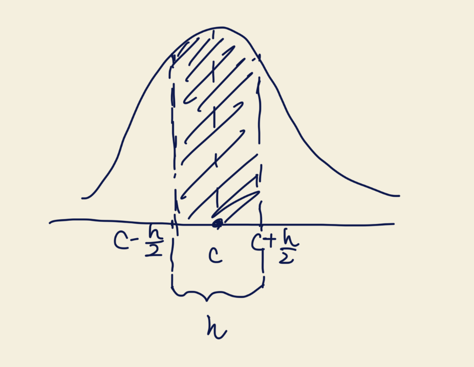
Rewrite

$$\begin{array}{rl}\widehat{f(c)}& =\frac{1}{nh}\sum _{i=1}^N\mathbb{I}\left\{c-\frac{h}{2}\le X_i\le c+\frac{h}{2}\right\}\\ & =\frac{1}{nh}\sum _{i=1}^N\mathbb{I}\{-\frac{1}{2}\le \frac{X_i-c}{h}\le \frac{1}{2}\}\\ & =\frac{1}{nh}\sum _{i=1}^N\mathbb{I}\{-\frac{1}{2}\le U_i\le \frac{1}{2}\}\end{array}$$

Where $U_i=\frac{X_i-c}{h}$. The meaning of $U_i$ is the relative distance between $X_i$ and $c$, scaled by the bandwidth $h$. Since we scale by $h$, no matter how we choose $h$, the interval $[c-h/2,c+h/2]$ always maps to $[-1/2,1/2]$ in the $U_i$ space.

Kernel Density Estimator

The above estimator is called the Histogram Density Estimator. It is simple but has some drawbacks, such as being discontinuous and sensitive to the choice of bandwidth. We replace the indicator function with a smooth function called a kernel function $K(\cdot )$, which satisfies:

$$\hat{f}(c)=\frac{1}{nh}\sum _{i=1}^{N}K\left(\frac{X_i-c}{h}\right)$$

Where $K(\cdot )$ is a kernel function that assigns weights to observations based on their distance from $c$. Common choices for $K(u)$ include:

1. Uniform kernel
2. Normal kernel
3. Epanechnikov kernel
4. Triangular kernel

It doesn’t matter which kernel function you choose, the results are often quite similar. The choice of bandwidth $h$ has a much larger impact on the estimate.

Properties: Mean, Variance, and Consistency

Mean

Note that:

$$\mathbb{E}[\hat{f}(c)]=\frac{1}{h}[K(\frac{X-c}{h})]$$

From the definition of expectation, we have:

$$\mathbb{E}[\hat{f}(c)]=\frac{1}{h}\int K(\frac{x-c}{h})f(x)dx$$

Let $u=\frac{x-c}{h}$, then $x=c+uh$ and $dx=hdu$. Thus:

$$\mathbb{E}[\hat{f}(c)]=\int K(u)f(c+uh)du$$

Using Taylor expansion, we have:

$$f(c+uh)=f(c)+f^{\prime }(c)uh+\frac{f^{\prime \prime }(c+h{u}^{\ast })}{2}(uh{)}^2$$

Here, we have an extra term $f^{\prime \prime }(c+h{u}^{\ast })$ instead of $f^{\prime \prime }(c)$ because of the Lagrange form of the remainder in Taylor expansion. It’s new to me as well, and from Claude it suggests that it’s another representation to capture the error term more accurately. i.e. $o(h^2)$.

Formally, the Largrangian form of the Taylor Expansion is:

$$f(c+uh)=f(c)+f^{\prime }(c)uh+\frac{f^{\prime \prime }(c+\theta \cdot hu)}{2}(uh{)}^2$$

Where $\theta \in (0,1)$. In this form, we let $\theta hu=h{u}^{\ast }$.

Back to our derivation, we have:

$$\mathbb{E}[\hat{f}(c)]=\int K(u)\{f(c)+f^{\prime }(c)uh+\frac{f^{\prime \prime }(c+h{u}^{\ast })}{2}(uh{)}^2\}du$$

Then we have:

$$=f(c)\int K(u)du+f^{\prime }(c)h\int uK(u)du+\int \frac{f^{\prime \prime }(c+h{u}^{\ast })h^2}{2}{u}^{2}K(u)du$$

Using the Condition of the Kernel Function:

1. $\int K(u)du=1$
2. $\int uK(u)du=0$ (The symmetric)
3. $\int u^{2}K(u)du=1$

We have:

$$=f(c)+0+\frac{h^2}{2}\int f^{\prime \prime }(c+h{u}^{\ast })u^{2}K(u)du$$

Focus on the last term, we have:

$$\int f^{\prime \prime }(c+h{u}^{\ast })u^{2}K(u)du=\int f^{\prime \prime }(c)u^{2}K(u))du+\int [f^{\prime \prime }(c+h{u}^{\ast })-f^{\prime \prime }(c)]u^{2}K(u)du$$

Simple Construction

We let the last term to be $2R_1$:

$$\int f^{\prime \prime }(c+h{u}^{\ast })u^{2}K(u)du=\int f^{\prime \prime }(c)u^{2}K(u))du+\underset{2R_1}{\underbrace{\int [f^{\prime \prime }(c+h{u}^{\ast })-f^{\prime \prime }(c)]u^{2}K(u)du}}$$

Thus we have:

$$\mathbb{E}[\hat{f}(c)]=f(c)+\frac{h^2}{2}\left[f^{\prime \prime }(c)+2R_1\right]$$

The last step is to prove that $R_1=o(1)$ as $h\to 0$.

Why we need to do so? Because if $R_1=o(1)$, then we have $\mathbb{E}[\hat{f}(c)]=f(c)+\frac{h^2}{2}{f}^{\prime \prime }(c)+o(h^2)$, which means our estimator is asymptotically unbiased.

Recall that:

$$R_1=\frac{1}{2}\int [f^{\prime \prime }(c+h{u}^{\ast })-f^{\prime \prime }(c)]u^{2}K(u)du$$

Our aim: prove that when $h\to 0$, $R_1\to 0$

Since from our condition, we have that $f^{\prime \prime }$ is continuous at $c$. By the definition of continuity, for any $ϵ>0$, there exists a $\delta >0$ such that if $|v|<\delta$, then $|f^{\prime \prime }(c+v)-f^{\prime \prime }(c)<ϵ$.

In other words, as long as $v$ is closed to $0$, then $f^{\prime \prime }(c+v)$ is closed to $f^{\prime \prime }(c)$.

We know that $|u|\le a$ because of the property of the kernel function: $K(u)=0$ when $|u|>a$. Thus, it is easy to have:

$$|h{u}^{\ast }|\le |hu|\le ha$$

We pick $h\le \delta /a$, then we have:

$$|h{u}^{\ast }|\le ha\le \delta$$

Since $|h{u}^{\ast }|<\delta$, we have:

$$|f^{\prime \prime }(c+h{u}^{\ast })-f^{\prime \prime }(c)|<ϵ$$

for all $|u|\le a$.

Now we are able to estimate $|R_1|$:

$$|R_1|=\left|\frac{1}{2}\int [f^{\prime \prime }(c+h{u}^{\ast })-f^{\prime \prime }(c)]u^{2}K(u)du\right|\le \frac{1}{2}\int |f^{\prime \prime }(c+h{u}^{\ast })-f^{\prime \prime }(c)||u^{2}K(u)|du$$ $$\le \frac{1}{2}\int ϵu^{2}K(u)du=\frac{ϵ}{2}\int u^{2}K(u)du=\frac{ϵ}{2}\cdot 1=\frac{ϵ}{2}$$

Since $ϵ$ is arbitrary, we have $R_1\to 0$ as $h\to 0$.

Thus we have shown that $R\to 0$ as $h\to 0$

$$\mathbb{E}[\hat{f}(c)]=f(c)+\frac{h^2}{2}{f}^{\prime \prime }(c)+o(h^2)$$

Variance

The method is similar to the derivation of mean.

We recall that $\hat{f}(c)=\frac{1}{nh}{\sum }_{i=1}^{N}K\left(\frac{X_i-c}{h}\right)$, and recall the definition of the variance: $\text{Var}[\hat{f}(c)]=\mathbb{E}[\hat{f}(c{)}^2]-\{\mathbb{E}[\hat{f}(c)]{\}}^2$

$$\begin{array}{rl}\text{Var}[\hat{f}(c)]& =\text{Var}[\frac{1}{nh}K(\frac{X-c}{h})]\\ & =\frac{1}{n{h}^2}\text{Var}[K(\frac{X-c}{h})]\\ & =\frac{1}{n{h}^2}\{\mathbb{E}[K(\frac{X-c}{h}{)}^2]-\mathbb{E}[K(\frac{X-c}{h}){]}^2\}\end{array}$$

Then we take the integral:

$$\mathbb{E}[K(\frac{X-c}{h}{)}^2]=\int K(\frac{x-c}{h}{)}^{2}f(x)dx$$ $$\mathbb{E}[K(\frac{X-c}{h}){]}^2=(\int K(\frac{x-c}{h})f(x)dx{)}^2$$

Similar to what we have done in the mean part, we let $u=\frac{x-c}{h}$, then $x=c+uh$ and $dx=hdu$. Thus:

$$\mathbb{E}[K(\frac{X-c}{h}{)}^2]=\int K(u{)}^{2}f(c+uh)hdu$$ $$\text{Var}[\hat{f}(c)]=\frac{1}{nh}\int K(u{)}^{2}f(c+hu)du-\frac{1}{n}{\left(\int K(u)f(c+hu)du\right)}^2$$

For simplification, we denote:

$$\text{Var}[\hat{f}(c)]=V_1-V_2$$

where $V_1=\frac{1}{nh}\int K(u{)}^{2}f(c+hu)du$ and $V_2=\frac{1}{n}{\left(\int K(u)f(c+hu)du\right)}^2$.

For $V_1$, using Taylor expansion, we have:

$$f(c+hu)=f(c)+f^{\prime }(c)hu+O(h^2)$$

Thus we have:

$$V_1=\frac{1}{nh}\int K(u{)}^2[f(c)+f^{\prime }(c)hu+O(h^2)]du$$ $$=\frac{1}{nh}\left[f(c)\int K(u{)}^{2}du+f^{\prime }(c)h\int uK(u{)}^{2}du+O(h^2)\right]$$

Since $\int uK(u{)}^{2}du=0$ (The symmetric), we have:

$$V_1=\frac{1}{nh}\left[f(c)\int K(u{)}^{2}du+O(h^2)\right]=\frac{f(c)}{nh}\int K(u{)}^{2}du+O(\frac{1}{n})$$

We could also follow the lecture slides where we let:

$$V_1=\frac{1}{nh}f(c)\int K(u{)}^{2}du+\frac{1}{nh}{R}_2$$

where $R_2=\int K(u{)}^2[f(c+hu)-f(c)]du$.

And we could also show that $R_2=o(1)$ as $h\to 0$ using the similar method in the mean part.

We skip the part of $V_2$ because the method is very similar. Finally we could have $O(n^{-1})=o(\frac{1}{nh})$

Consistency

We finally could have:

$$\begin{array}{r}\mathbb{E}[\hat{f}(c)]\to f(c)\\ \\ \text{Var}[\hat{f}(c)]\to 0\end{array}$$

Since convergence in mean square implies convergence in probability, we have:

$$\hat{f}(c){\to }^{p}f(c)$$