Exponential Smoothing

Time-Series Components

This is typically compared with the Moving Averages, because the moving average has some huge disadvantages that it will lose the first and last sets of time periods. If the time-series only has a few observations, it could lose some important information (for example, only 5 years?)

The second reason is that the Moving Averages method will ignore a lot of previous observation / information.

But, we can use the Exponential Smoothing method to solve this problem! In conclusion, we have

$S_t=w{y}_t+(1-w)S_{t-1}fort\ge 2$

where $S_t$ is Exponentially smoothed time series at time period $t$ $y_t$ is the time series at time period t $w$ is the smoothing constant

You can understand the $S_t$ as a $y_t^{\prime }$ ,which means it is after a smoothing procedure. And, if we start from $t=1$, we could get $S_t=w{y}_t+(1-w)y_{t-1}+w(1-w{)}^2{y}_{t-2}+...+(1-w{)}^{t-1}$

There is no $w$ in the last component. See it carefully.

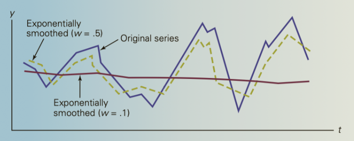
Different choose of value $w$ could change the deal of smoothing. Normally a large value of $w$ could has a little smoothing, vice versa.

附上 R 语言代码：

library(forecast)
library(ggplot2)
# 加载数据
sales <- c(39, 37, 61, 58, 18, 56, 82, 27, 41, 69, 49, 66, 54, 42, 90, 66)
 
# 定义指数平滑系数alpha
w1 <- 0.2
w2 <- 0.7
 
# 计算初始的预测值
pred1 <- sales[1]
pred2 <- sales[1]
# 进行指数平滑处理
for (i in 2:length(sales)) {
  pred1[i] <- w1 * sales[i] + (1 - w1) * pred1[i-1]
}
for (i in 2:length(sales)) {
  pred2[i] <- w2 * sales[i] + (1 - w2) * pred2[i-1]
}
 
 
sales_df <- data.frame(
  Month = 1:16,
  Sales = sales,
  Prediction1 = pred1,
  Prediction2 = pred2
)
# 输出预测结果
print(pred1)
print(pred2)
ggplot(data = sales_df, aes(x = Month)) +
  geom_line(aes(y =sales , color = "red"),size = 1)+
  geom_line(aes(y =pred1 , color = "blue"), size = 1, linetype = "dashed")+
  geom_line(aes(y =pred2))