EC423 Review

EC423 复习笔记

Material Scan

Found in EC423 Labour/:

Category	Materials found	How used
Lecture slides	Lecture Slides/EC423_Autumn_Topic1-4.pdf; Lecture Slides/EC423_WT_Lec1-10.pdf; EC423_WT_Lec4_Update.pdf	主干来源；冬季 Lecture 4 采用 update 版
Reading list	Reading List.pdf	用于核对冬季 Topic 顺序与核心 readings
Problem sets	Problem Sets/PS_1_labor_supply.pdf, PS_2_card_robins.pdf, PS_3_ret_to_schooling.pdf, EC423_PS4.pdf, PS_5_roy.pdf, PS_6_katz_murphy.pdf, winter analytical/applied problem sets	只提取考法、推导套路、实证设计，不代写答案
Solutions	Seminar/solutions/PS_1_labor_supply_solutions.pdf	用于校准劳动供给推导
Seminars	Seminar/EC423_AT_Seminar_1-2.pdf, Seminar/EC423_WT_Seminar_1.pdf, Seminar/EC423_WT_Seminar_3.pdf	用于补充方法论与 problem-set 推导路径
Past exams	Past Exams/EC423_2020-2025.pdf	用于识别反复出现的题型
Other	Sample Exam Questions.pdf text extraction was blank; AT/ contains duplicate/essay material	未作为主干证据

Omitted Variable Bias: 并不是越多的控制变量 $X$ 越好。有两个因素：

1. Bad Control 问题：如果 $X$ 是某一个 post 后验的变量，即 $X$ 受 $D$ 是否接受 treatment 的影响，那么 $X$ 就是一个 bad control。原则是：只能控制不受 treatment 影响的变量（pre-treatment 或 predetermined 的变量）
2. CIA 假设可能仍然不成立：即使你加了很多 $X_i$ ​，只要还有遗漏的、同时与 $D_i$ ​ 和 $Y_i$ 相关的变量，OVB 就依然存在。你永远无法确定自己已经控制了”所有”相关变量，这也是为什么课程更强调 IV、DiD、RDD 这些基于研究设计的方法——它们不依赖于”控制了足够多变量”这个很强且不可检验的假设。

如何判断 OLS bias 的方向： 方法就是把 OVB 公式 ${\beta }_s=\beta +{\gamma }^{\prime }{\delta }_{XD}$ 拆成两个符号的乘积：

以大学毕业（college graduation）作为被省略变量为例：

• $\gamma$：大学毕业对工作时间的影响 → 大概率是正的（受教育更多的女性倾向于工作更多）
• ${\delta }_{XD}$：大学毕业与生第三个孩子的关联 → 大概率是负的（受教育越多越倾向于少生）

所以偏误 ${\gamma }^{\prime }{\delta }_{XD}<0$，意味着 ${\beta }_s<\beta$。由于 $\beta$ 本身就是负的（生孩子减少工作时间），${\beta }_s$ 比真实效应更负——OLS 会夸大孩子对劳动供给的负面影响。

Slides 还提到可以用 potential outcomes 的语言理解同样的事情：$E[Y_{0i}|D_i=1]-E[Y_{0i}|D_i=0]<0$，即有孩子的女性即使不生孩子也会比无孩子女性工作得少（因为她们教育程度更低等），这就是 negative selection bias，与上面 OVB 分析的结论一致。

核心技巧就是：分别判断两个分量的符号，然后相乘，就能知道偏误方向。

Autumn Topic 1: Labor Supply and Welfare Systems

Key Concepts

Definition

静态劳动供给模型 (static labor supply model)：个人在消费 $x$ 与 leisure $\ell$ 之间选择，$h=T-\ell$，预算约束为 $px=wh+y$ 或 $px+w\ell =wT+y$，其中 $wT+y$ 是 full incomeAT Topic 1 课件页 7-13。

Intuition

工资既是工作一小时的收入，也是 leisure 的机会成本；因此工资变化会同时改变相对价格和实际购买力，这就是劳动供给符号不确定的根源AT Topic 1 课件页 20-23。

Formula

内点解一阶条件：$\frac{u_{\ell }(x,T-h)}{u_x(x,T-h)}=\frac{w}{p}$。左边是个人用 leisure 换消费的边际替代率 (MRS)，右边是市场交换率AT Topic 1 课件页 11-12｜推荐练习：PS1 Q1a。

Intuition

最优点不是“想多休息”或“想多消费”的单边选择，而是让主观 trade-off 等于市场 trade-off；若 MRS 高于工资，leisure 对个人太贵，应该多工作AT Topic 1 课件页 12。

Formula

Slutsky equation for labor supply：Marshallian wage effect = compensated substitution effect + income effect. 课件用 leisure/labor duality 推出：补偿劳动供给对工资的反应为正；若 leisure 是 normal good，收入效应使工作时间下降AT Topic 1 课件页 17-23。

Intuition

工资上升让 leisure 更贵，所以 substitution effect 推动多工作；但工资上升也让同样工作时间带来更高收入，所以 income effect 推动多休闲。两者方向相反，因此 uncompensated labor supply 可能向上也可能向后弯曲AT Topic 1 课件页 21-23。

Definition

非参与与 reservation wage：如果市场工资低于个人进入劳动市场所要求的保留工资，最优选择在角点 $h=0$；Heckman-style selection 问题来自我们只在就业者身上观察工资或工时AT Topic 1 课件页 46-53。

Intuition

工资数据不是随机抽来的“所有人潜在工资”，而是已选择工作的人；如果选择工作本身与未观测能力、偏好或家庭约束相关，简单 OLS 会混入选择偏差AT Topic 1 课件页 49-53。

Taxes, Transfers, And Welfare Systems

Formula

加入税收、福利和固定工作成本后，预算约束可写为 $C=Y+1(H\le 0)\cdot welf+w(T-L)(1-\tau )-1(H>0)\cdot LC$；预算线出现 kink 与 non-convexity，FOC 不再够用AT Topic 1 课件页 62-64。

Intuition

福利制度经常改变的不只是斜率，还会制造进入工作的固定成本或门槛；这使 extensive margin 的参与决策比内点工时选择更重要AT Topic 1 课件页 62-66。

Definition

Income floor：政府保证最低收入 $G$。其效果可能使低收入者退出工作，也可能把部分人留在 kink；静态模型需要分 initial hours 场景讨论AT Topic 1 课件页 65-66｜推荐练习：Exam 2021 Q2, Exam 2025 Q2。

Intuition

收入底线像给低收入者一段“平的预算线”：低工时工作不增加收入，因此工作激励弱；但对原本无收入的人，它提高保障，福利改善不等于劳动供给增加AT Topic 1 课件页 65-66。

Formula

Negative Income Tax (NIT)：含 guarantee $G$ 与 tax rate $t$；课件给出的总效应为 $dh=\frac{\partial h}{\partial w}{|}_U(-tw)+\frac{\partial h}{\partial M}[h(1-t)w+G]$，若 leisure 为 normal good，两个项都推低劳动供给AT Topic 1 课件页 67-72。

Intuition

NIT 同时降低边际工作回报并提高非劳动收入，所以 substitution 和 income channels 同向压低工时；这解释了福利国家在 redistribution 与 work incentives 之间的基本 trade-offAT Topic 1 课件页 70-71。

Empirical Evidence And Identification

Example

Lottery evidence：Imbens et al. 与 Swedish lottery data 用随机奖金识别 wealth/income effect；瑞典研究通过 lottery cell fixed effects 与 pre-lottery covariates 检验随机化，并分解 earnings response 为 hours 与 wagesAT Topic 1 课件页 24-45｜推荐练习：Exam 2024 Q1。

Intuition

彩票奖金近似随机改变 non-labor income，因此主要对应 Slutsky 中的收入效应；分解 hours/wages 是为了判断收入下降来自少工作，还是选择了不同工资的工作AT Topic 1 课件页 38-45。

Example

Self-Sufficiency Project (SSP)：随机 offer wage supplement，要求 30 小时以上工作并退出 welfare；平均工时 treatment-control gap 随 quarter 上升，PS2 要求把静态劳动供给图和实际动态 response 对照AT Topic 1 课件页 75-87｜推荐练习：PS2 Q1, Exam 2023 Q2。

Intuition

SSP 的门槛制造强烈 extensive-margin incentive：一部分人会从不工作或低工时跳到 30 小时附近；但动态效果还取决于 take-up、信息、找工作摩擦和 program expiration，静态模型无法单独预测时间路径AT Topic 1 课件页 75-87。

Causal Inference: OLS, OVB, IV, LATE

Formula

Omitted Variables Bias：短回归遗漏与处理变量相关、且影响 outcome 的变量时，OLS 估计等于 causal effect 加上 selection term；课件用 children 对女性劳动供给的例子说明 OLS 估计 ATT/ATE 都可能失败AT Topic 1 课件页 100-123。

CIA

即 Conditional Independence Assumption

要注意辨析：“生不生孩子都不会影响这个人的 outcome”在字面上是说：

$Y_{1i}-Y_{0i}=0$

即 treatment 对 outcome 没有因果效应。

而 CIA 说的是：

$E[Y_{0i}\mid X_i,D_i=1]=E[Y_{0i}\mid X_i,D_i=0]$

即条件于 $X_i$，生与不生的两组人在基准水平上没有差异，但生孩子本身仍然可以对每个人的 outcome 产生很大影响。

如果你想用中文准确表述 CIA，可以说：固定 $X_i$ 后，生不生孩子这个”选择”与这个人本身会工作多少无关——而不是说生孩子这件事不影响工作时数。

区别在于：“选择谁进入 treatment”与 potential outcomes 无关 vs “treatment 本身对 outcome 没影响”。前者是 CIA，后者是零效应。

Intuition

有孩子的女性和没孩子的女性不只差在孩子数量，也可能差在偏好、职业路径、家庭结构；OLS 比较的是“孩子效应 + 原本就不同”的混合物AT Topic 1 课件页 104-123。

Definition

IV 需要 first stage 与 exclusion restriction；Angrist and Evans 使用前两个孩子同性作为第三胎的 instrument，2SLS 只使用由性别组合诱发的 fertility variationAT Topic 1 课件页 124-133。

Intuition

好 IV 像一个只推动 treatment、不直接碰 outcome 的外部拨杆；如果拨杆还通过其他路径影响 outcome，exclusion restriction 断裂AT Topic 1 课件页 125-128。

Formula

LATE theorem：在 independence、exclusion、first stage、monotonicity 下，binary-IV Wald ratio 识别 compliers 的平均处理效应 $E[Y_1-Y_0\mid D_1=1,D_0=0]$AT Topic 1 课件页 134-149。

Local Average Treatment Effect

Intuition

IV 估计的不是全体平均效应，而是“会被 instrument 推动改变 treatment 状态的人”的效应；这解释了为什么强 first stage 和清楚的 complier 描述在考试答案里很重要AT Topic 1 课件页 142-149。

Problem Patterns

Example

常考推导：给定 $U(c,\ell )=c^{\alpha }\ell$，推出 $h=\frac{\alpha wT-y}{(1+\alpha )w}$、uncompensated/compensated wage elasticity，并解释 overtime premium；seminar solution 显示 $T=80,y=0,\alpha =1$ 时 $h^{\ast }=40$，若 $h^{\prime }=h^{\ast }/4$ 需 $w^{\prime }=2w$ PS1 Q1 PS1 solutions 页 1-3 AT Seminar 2 页 29-71。

Technique

UBI/income floor 题不要只画一条预算线。分三步写：初始是否工作、是否在 eligibility threshold 附近、政策是否改变 slope 或 intercept；2021 与 2025 都几乎原样考 UBI vs income floorExam 2021 Q2``Exam 2025 Q2。

Autumn Topic 2: Human Capital

Mincer Model

Definition

Human capital：可提高劳动市场产出与 earnings capacity 的技能、教育、经验和健康等；Becker 区分 general 与 specific human capitalAT Topic 2 课件页 2-8。

Intuition

人力资本把教育从消费品变成投资品：教育的成本是学费和放弃工资，收益是未来工资流上升AT Topic 2 课件页 9-15。

Formula

Mincer 模型假设固定劳动供给、上学期间无收入、无退休、完美信贷市场且教育唯一成本为 foregone earnings；最大化 lifetime earnings 后，FOC 可写为 $\partial \log y/\partial S=r$AT Topic 2 课件页 9-16｜推荐练习：PS3 Q1。

Intuition

继续上学直到边际教育回报等于贴现率；若回报高于 $r$，推迟工作值得，若低于 $r$，应进入劳动市场AT Topic 2 课件页 14-17。

Warning

简单 Mincer 回归 $\log w_i=\alpha +\rho S_i+X_i^{\prime }\beta +{\epsilon }_i$ 的 $\rho$ 不自动等于 causal return。ability bias、measurement error、family background、health controls 是否 bad controls 都要讨论AT Topic 2 课件页 30-42｜推荐练习：EC423_PS4 Q7。

Intuition

如果能力高的人既更可能多读书又工资更高，教育系数会吸收能力；如果控制变量本身是教育的结果，例如健康或职业选择，就可能把教育效应的一部分控制掉AT Topic 2 课件页 30-42``EC423_PS4 页 1-2。

Returns To Schooling And IV

Example

Angrist and Krueger 的 quarter-of-birth IV 使用 compulsory schooling law 产生教育年限差异；关键是出生季度影响教育，但不应直接影响工资AT Topic 2 课件页 43-52。

Intuition

IV 把教育选择中由能力、家庭背景导致的内生部分剥离，只保留制度规则造成的 schooling variation；但若出生季度与家庭季节性、健康、年龄入学等直接相关，exclusion 会受威胁AT Topic 2 课件页 44-52。

Difference-In-Differences

Definition

Difference-in-Differences (DiD)：假设无处理时 treatment-control 差异随时间保持常数；估计 $\{E[Y|T,post]-E[Y|T,pre]\}-\{E[Y|C,post]-E[Y|C,pre]\}$AT Topic 2 课件页 55-64。

Intuition

control group 的变化估计“正常时间变化”，treated group 的额外变化才归因于政策；识别靠 parallel trends，而不是水平相同AT Topic 2 课件页 57-65。

Warning

Ashenfelter’s dip：若 treatment group 在政策前就因负面冲击而下滑，pre-post recovery 会被误认为 treatment effect；多期数据应画 event-study/pre-trendsAT Topic 2 课件页 65-68。

Intuition

DiD 最怕“被治疗”本身是坏趋势的结果；培训项目、最低工资、地方政策都常见这种选择进入问题AT Topic 2 课件页 65-73。

Warning

staggered DiD with heterogeneous effects 可能出现 negative weights；若所有 cell 的 ATE 都为正，TWFE 仍可能估出负数AT Topic 2 课件页 69-72。

Intuition

旧 TWFE 把已处理组当别人的 control，会在 treatment timing 不同且 effect 动态变化时扭曲权重；考试中提到要用 cohort/event-time robust estimators 会很加分AT Topic 2 课件页 69-72。

Regression Discontinuity

Definition

Sharp RD：处理 $D_i=1(x_i\ge x_0)$ 由 running variable 的阈值确定；识别 cutoff 附近 treatment effectAT Topic 2 课件页 74-80。

Intuition

阈值两边很近的人应当相似，除了是否刚好拿到政策；RD 是 local comparison，不是全样本平均效应AT Topic 2 课件页 74-81。

Formula

线性 sharp RD 可估 $Y_i=\alpha +\beta x_i+\rho D_i+{\eta }_i$；非线性时需允许 $E[Y_0|x]$ 与 $E[Y_1|x]$ 平滑但不一定线性，避免把曲线错当 jumpAT Topic 2 课件页 80-86。

Intuition

RD 的因果识别来自“离散跳跃”，不是整体斜率；若 counterfactual CEF 本身有 sharp curvature，高阶多项式可能制造假跳跃AT Topic 2 课件页 81-88。

Technique

RD 检查：pre-treatment covariates 在 cutoff 处不能跳；running variable density 不能在 cutoff bunching，McCrary test 常用于 manipulation checkAT Topic 2 课件页 91-95｜推荐练习：Exam 2020 Q2, Exam 2022 Q2。

Definition

Fuzzy RD：threshold 只造成 treatment probability 的跳跃，使用 threshold indicator 作为 IV；Wald ratio 识别 cutoff 附近 compliers 的 treatment effectAT Topic 2 课件页 96-101。

Intuition

fuzzy RD 的“被阈值推动接受处理的人”就是 local compliers；因此外推到远离 cutoff 的人要非常谨慎AT Topic 2 课件页 100-101。

Problem Patterns

Example

PS3 要求从 continuous-time schooling choice 推出 $\partial \log y/\partial S=r$，分析 ability $A$、schooling cost/subsidy 与 wage $w$ 对最优 schooling 的影响PS3 Q1。

Example

EC423_PS4 是 Mincer 回归实操：构造 log hourly wage、schooling、age/age squared、parental schooling、female、AFQT、health limitation，并比较 schooling coefficient 随 controls 变化EC423_PS4 页 1-2。

Autumn Topic 3: Immigration

主要探讨两个话题：Effects of immigrants on natives and Selection of immigrants (Roy Model)

A migrant 移民者 is simply defined as a person born in a country but different from where they are currently living.

Immigration Surplus

Definition

简单 immigration model：生产函数 $Y=F(K,N+M)$，CRS、完全竞争、劳动无弹性、短期资本固定；移民增加 $M$AT Topic 3 课件页 15-18。

Formula

Immigration surplus result：本地人总收入为 $Y-WM$；在 CRS 与完全竞争下，移民增加使 natives average income 上升，但劳动者与资本所有者分配不同AT Topic 3 课件页 16-21。

详细手写推导见 p18

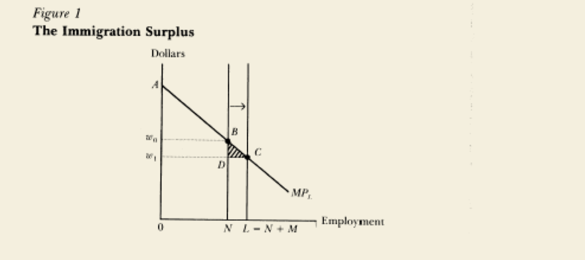
Intuition

新移民压低边际劳动产品工资，但也扩大总产出；资本和互补要素获得的增益可以超过原生劳动者工资损失，所以总 native surplus 为正但分配冲突尖锐AT Topic 3 课件页 17-20。

Warning

异质劳动下没有简单总结果。若 skilled immigration 增加，native income 是否上升取决于移民在各技能组中的占比和跨技能替代/互补关系AT Topic 3 课件页 22-27。

Otherwise lead to workers lose, capitalists gain problem.

Intuition

“移民影响工资”不是一个单一参数：如果移民与某些 natives 是 substitutes，他们可能压低该组工资；若与另一些 natives 是 complements，反而提高其 marginal productAT Topic 3 课件页 22-28。

Definition

Another Approach would be Immigration with heterogeneous labour, assume there are two types of labor, high skill and low skill, the production function now becomes:

F(N_{1}+M_{1}, N_{2}+M_{2}) = F(L_{1},L_{2})$$ Constant Return to Skill arguments:

F(L_{1},L_{2}) = L_{2} f\left( \frac{L_{1}}{L_{2}} \right)

然后可以通过求导算出 $w_1,w_2$ 。接下来考虑一个场景即，高技能的工人涌入，也就是说带来了 $M_1$ .

最后的结论是， immigration of type 1 labour will raise income of natives if:

$$\frac{M_1}{L_1}>\frac{M_2}{L_2}$$

i.e. share of migrants in type 1 labour is higher than share in type 2 labour.

Empirical Approaches

Example

David Card (1990), “The Impact of the Mariel Boatlift on the Miami Labor Market.”

主要内容：这篇论文研究的是：1980 年 Mariel Boatlift 这次大规模古巴移民冲击，对 Miami 本地劳动市场有什么影响。

背景是：1980 年 Castro 突然允许古巴人从 Mariel 港口离开；1980 年 5 月到 9 月，约 125,000 名古巴移民抵达 Miami，其中约一半永久定居在 Miami。这使 Miami 劳动力规模上升约 7%，古巴工人数量上升约 20%。

Identification Strategy: 核心识别思路是把 Mariel Boatlift 当作一个 plausibly exogenous immigration shock。 可以把它理解成一种 local labour market natural experiment / difference-in-differences-style comparison：

Miami after 1980−Miami before 1980

再和没有受到 Mariel shock 的 comparison cities 比较。

识别假设是：如果没有 Mariel Boatlift，Miami 的 low-skilled labour market trend 会和 comparison cities 类似。

Card 结论是：Mariel immigration 对 Miami non-Cuban workers 的 wages 或 employment outcomes 没有明显影响。

课件还强调，Miami 古巴工人平均工资在 1980 后下降，但这个下降并不超过“把收入较低的新 Mariel immigrants 加入 Cuban worker pool”后本来就会机械产生的下降。

Intuition

移民冲击难点在 counterfactual：接收城市可能本来趋势不同，本地人和资本会迁移，产业结构会调整；因此估计值往往是 local/general-equilibrium 混合效应AT Topic 3 课件页 37-46。

另一个非常有意思的感悟：几乎所有的 natural experiment 似乎都可以用 External Validity 去 challenge，因此也许可以视作一个考试通解。

Example

Doran 2011: The Collapse of the Soviet Union and the Productivity of American Mathematicians.

这篇研究的是：高技能移民冲击对本地高技能 workers 的影响。主要想探究这些顶尖数学家对美国本土的科研人员是 complements 还是 substitute?

Identification Strategy: field exposure DiD。不是所有美国数学领域都受到同样冲击。苏联数学家在某些 subfields 很强，所以这些领域在苏联解体后突然收到大量高技能竞争者；其他领域受到的冲击较小。课件说，可以比较美国数学家对 Soviet mathematicians 的不同 exposure。通过构建 exposure index，直觉是：如果一个美国数学家原本研究的领域和苏联数学家的优势领域高度重合，他受到的 Soviet supply shock 更大。课件还列了 intensity index 和 similarity index。

结果是：受 Soviet mathematicians 冲击更大的美国数学家，之后 publication 和 citations 明显下降。

这个 paper 的核心信息是：高技能移民不一定只带来 knowledge spillovers；在某些专业市场里，他们也可能和本地高技能 workers 直接竞争。

Roy/Borjas Selection Model

了解 self-selection 是非常重要的话题。

Definition

Roy model：个体在多个 sector/country 中选择收益最高者，观察到的 sector earnings 是选择后的结果，不能直接当作 treatment effectAT Topic 3 课件页 47-54。

Intuition

移民不是随机抽样的人；他们是“在源国与目的国收益差、迁移成本、技能回报结构”下选择迁移的人，所以 observed immigrant earnings 同时反映 selection 与 treatment effectAT Topic 3 课件页 51-59。

Formula

Borjas setup：源国 $w_0={\mu }_0+{\epsilon }_0$，目的国 $w_1={\mu }_1+{\epsilon }_1$，迁移成本 $C=\pi \exp (w_0)$；迁移条件近似为 $({\mu }_1-{\mu }_0-\pi )+({\epsilon }_1-{\epsilon }_0)>0$，令 $\nu ={\epsilon }_1-{\epsilon }_0$AT Topic 3 课件页 56-63｜推荐练习：PS5 Q1, Exam 2020 Q1, Exam 2023 Q1。

Intuition

迁移概率随目的国平均收益上升而上升，随源国平均收益与迁移成本上升而下降；但谁迁移还取决于两国技能回报的方差与相关性AT Topic 3 课件页 61-69。

Definition

Inverse Mills Ratio (IMR) 用来计算截断正态下的选择项，例如 $E[{\epsilon }_0\mid \nu /{\sigma }_{\nu }>z]$；它衡量“进入迁移样本”后未观测能力的条件均值AT Topic 3 课件页 64-68。

Probability of Migration:

$$\begin{array}{rl}P& =\mathbb{P}[v>({\mu }_0-{\mu }_1+\pi )]\\ & =\mathbb{P}\left[\frac{v}{{\sigma }_v}>\frac{({\mu }_0-{\mu }_1+\pi )}{{\sigma }_v}\right]\\ & =1-\Phi (\frac{({\mu }_0-{\mu }_1+\pi )}{{\sigma }_v})\\ & =1-\Phi (z)\end{array}$$

Intuition

如果只观察迁移者，样本左/右尾被筛选；IMR 是把“被筛进样本的未观测成分”显式写出来，避免把选择效应误认为迁移收益AT Topic 3 课件页 64-68。

Definition

Selection cases：positive hierarchical sorting 可理解为 best and brightest migrate；negative hierarchical sorting 是低技能被高压缩工资结构吸引；refugee sorting 是源国底部但目的国顶部的人迁移AT Topic 3 课件页 69-75。

Intuition

同一迁移流可能是 brain drain、insurance-seeking migration 或 refugee sorting；关键不是“移民高/低技能”，而是技能在源国与目的国的回报排序是否一致AT Topic 3 课件页 70-75。

Autumn Topic 4: Inequality And Technological Change

Stylized Facts And Quantiles

Definition

Inequality facts：美国和多国收入/工资不平等上升，劳动份额下降，top income shares 上升；1990s 后出现 polarization，即中间岗位相对下降AT Topic 4 课件页 2-28。

Intuition

平均工资无法描述“谁受益、谁受损”；技术变化、教育供给和制度变化可能同时提高上尾、压低中间或改变 lower tailAT Topic 4 课件页 20-30。

Definition

Quantile regression (QR)：估计 $Y$ 条件分布的某个分位数而不是条件均值；loss function ${\rho }_{\tau }(u)$ 是不对称绝对损失，$\tau =.5$ 时对应 medianAT Topic 4 课件页 29-39。

Intuition

QR 回答“给定 $X$，分布第 $\tau$ 分位在哪里”，不是“某个原来处于第 $\tau$ 分位的人会怎样”；除非 rank-preserving，否则不能把分布效应直接当个体效应AT Topic 4 课件页 39-42。

Definition

Quantile Treatment Effect (QTE)：把因果问题扩展到结果分布；Abadie, Angrist, and Imbens QTE 与 LATE 的假设结构相近AT Topic 4 课件页 42-45。

Intuition

政策可能均值不变但 lower tail 改善或 upper tail 受损；QTE 在 inequality 题中很有用，因为它直接考察分布形状变化AT Topic 4 课件页 42-45。

CES Skill Premium

Definition

CES framework：$Y=[(A_{L}L{)}^{\rho }+(A_{H}H{)}^{\rho }{]}^{1/\rho }$，$L$ 为 low-skilled，$H$ 为 high-skilled，$\sigma =1/(1-\rho )$ 是 substitution elasticityAT Topic 4 课件页 57-60｜推荐练习：PS6 Q1, Exam 2024 Q2。

Intuition

$\sigma$ 决定技能组是更像 substitutes 还是 complements；它控制教育供给扩张或 skill-biased technology 对 skill premium 的强度AT Topic 4 课件页 58-61。

Formula

完全竞争下工资等于边际产品；CES 推出 own labor demand downward sloping，同时 $\partial W_H/\partial L>0$、$\partial W_L/\partial H>0$，即 Q-complementarityAT Topic 4 课件页 63-66。

Intuition

一个技能组数量上升会降低自身边际产品，但可能提高另一技能组边际产品；这就是为什么高技能供给扩张不一定伤害低技能工资AT Topic 4 课件页 64-66。

Formula

Skill premium 由相对技术 $A_H/A_L$ 与相对供给 $H/L$ 共同决定；Katz and Murphy 估计式中 time trend 捕捉 relative demand trend，relative supply 系数估计 $-1/\sigma$，得到 $\sigma \approx 1.4$AT Topic 4 课件页 65-77｜推荐练习：PS6 Q1。

Intuition

1940-2000 年间 skilled relative supply 和 skill premium 同升，说明 relative demand for skill 也在上升；这就是 Tinbergen/Goldin-Katz “race between education and technology”AT Topic 4 课件页 71-79。

Warning

Aggregate time-series 估计 $\sigma$ 有样本少、serial correlation、相对供给内生性等问题；2024 考题要求用 aggregate data 和 firm panel data 分别讨论识别假设Exam 2024 Q2。

Robots And Future Of Work

Example

课件讨论 industrial robots 的测量与对 productivity、wages、employment 的影响，强调从相关性走向因果识别需要行业-国家-时间的 exposure variationAT Topic 4 课件页 83-90。

Intuition

技术冲击不只是“机器替代人”；它可能提高生产率、改变任务分配、改变技能需求，也可能通过产品市场扩张抵消直接替代效应AT Topic 4 课件页 83-93。

Winter Lecture 1: Gender Inequality

Facts And Child Penalty

Definition

Gender gaps：女性劳动参与率长期上升，女性人力资本投资平均不低于男性，但 gender wage gap 仍广泛存在并随 cohort 下降WT Lec 1 课件页 7-25。

Intuition

“教育差距”已经不能解释全部性别工资差距；现代核心机制转向 child penalty、hours/occupation adjustments、firm frictions、norms 与 discriminationWT Lec 1 课件页 26-55。

Example

Bertrand, Goldin & Katz MBA study：男女 MBA 初始 earnings 相近，但十年后男性优势可达约 60 log points，机制包括 training、career interruptions 与 weekly hoursWT Lec 1 课件页 29-38。

Intuition

高回报职业通常对连续工作和长工时有非线性奖励；child-related interruptions 因此会被放大成长期 earnings gapWT Lec 1 课件页 31-38。

Example

Kleven, Landais and Sogaard child penalty：女性生育后 earnings、hours、participation 和 occupational rank 显著下降，且 child-related inequality 持久WT Lec 1 课件页 39-54。

Intuition

child penalty 是事件研究逻辑：生育前男女轨迹相近，生育后女性偏离；它把“性别差距”定位到家庭形成时点的劳动供给和职业调整WT Lec 1 课件页 39-54。

Household Labor Supply Model

Formula

Olivetti-Pan-Petrongolo household model：$U=m^{1-\theta }{H}^{\theta }$，$w_m=p_m$，$w_f=\varphi p_f$，$H=(1-h_f{)}^{\eta }(1-{\bar{h}}_m{)}^{1-\eta }$；$\varphi <1$ 表示 markdown/frictions/discrimination，$\eta$ 表示 wife time 在 home production 中的重要性WT Lec 1 课件页 56-59。

Intuition

该模型把性别差距拆成 productivity、preferences、wage markdowns 与 norms 四类机制；同样 productivity 下，norms 和 frictions 也会降低女性参与和工时WT Lec 1 课件页 56-63。

Formula

Reservation wage：$w_R=\frac{\theta }{1-\theta }\eta w_m{\bar{h}}_m$；若 $w_f=\varphi p_f<w_R$，妻子不参与劳动市场WT Lec 1 课件页 60。

Intuition

家庭越重视 home time、妻子时间越被 normatively 绑定到家务、丈夫收入越高，女性 market work 的机会成本越高，参与门槛越高WT Lec 1 课件页 60。

Formula

若 $w_f\ge w_R$，女性最优市场工时 $h_f^{\ast }$ 随 $p_f$ 上升、随 markdown $\varphi$ 下降、随 $\theta$ 或 $\eta$ 上升而下降WT Lec 1 课件页 61-62。

Intuition

even conditional on working，norms 和 frictions 仍会降低 intensive margin；因此政策不能只看 participation，还要看 hours、occupation、firm sortingWT Lec 1 课件页 61-63。

Winter Lecture 2: Racial Inequality And Discrimination

Measurement And Oaxaca-Blinder

Definition

Racial disparities 可用 wage/employment/wealth/incarceration/mobility gaps 描述，但 racial classification 本身可能 endogenous，且 controls 可能是 discrimination 的结果WT Lec 2 课件页 4-29。

Intuition

控制变量越多不一定越“公平”：若 schooling、AFQT、criminal record 是早期歧视或环境差异造成的，控制它们会把结构性渠道拿掉WT Lec 2 课件页 18-37。

Definition

Oaxaca-Blinder decomposition 将 mean wage gap 分成 observable characteristics 差异解释的部分与 coefficients/returns 差异解释的 unexplained 部分WT Lec 2 课件页 45-49。

Intuition

“unexplained” 不是 discrimination 的机械同义词；它还包括遗漏变量、测量误差和模型设定问题，但它提示了 returns/valuation 差异的重要性WT Lec 2 课件页 45-49。

Taste-Based Discrimination

Definition

Becker taste-based discrimination：雇主有 prejudice parameter $d>0$，把雇佣 minority worker 的成本看成 $w_B+d$；雇主雇佣 $B$ 当且仅当 $w_W-w_B\ge d$WT Lec 2 课件页 57-62｜推荐练习：WT Analytical PS I Part II。

Intuition

prejudice 像对 minority labor 征税；若不歧视雇主足以吸纳全部 minority workers，均衡工资差可为零，工资差由 marginal discriminator 而非 average prejudice 决定WT Lec 2 课件页 60-65。

Formula

短期均衡中 marginal discriminator 满足 $w_W^{\ast }=w_B^{\ast }+d^{\ast }$；若 prejudiced firms 足够多，$B$ workers 被排序到较不歧视雇主，工资 gap 出现WT Lec 2 课件页 60-65。

Intuition

少数雇主歧视不必然导致工资差，关键是无偏见雇主的 demand 相对 minority labor supply 是否足够大WT Lec 2 课件页 61-65。

Statistical Discrimination

Definition

Statistical discrimination：雇主不完全观察 productivity $p_i$，用 noisy signal ${\tilde{p}}_i=p_i+v_i$ 与 group prior ${\bar{p}}_g$ 做 Bayesian updatingWT Lec 2 课件页 71-80｜推荐练习：WT Analytical PS I Part I, WT Seminar 3。

Formula

Signal extraction：$E(p_i\mid {\tilde{p}}_i,g)=(1-\beta ){\bar{p}}_g+\beta {\tilde{p}}_i$，其中 $\beta =\frac{{\sigma }_g^2}{{\sigma }_g^2+{\sigma }_v^2}$WT Lec 2 课件页 80-85。

Intuition

信号越 noisy，雇主越依赖 group mean；信号越精确，雇主越相信个人信息，group identity 的作用下降WT Lec 2 课件页 80-85。

Definition

Phelps cases：不同 group means 且同方差时，同一 signal 下低 prior group 工资更低；相同 means 但 signal precision 不同，也会使同一 signal 的 wage schedule 不同WT Lec 2 课件页 84-89。

Intuition

statistical discrimination 可以是“理性推断”但仍不公平；它会把群体历史差异转化为个人当下待遇差异，并可能自我强化WT Lec 2 课件页 84-90。

Formula

Altonji-Pierret test：$\ln w_{it}=\gamma E_{it}+\theta T_i+\delta S_i+{\beta }_1(T_i\times E_{it})+{\beta }_2(S_i\times E_{it})+\eta X_{it}+{\epsilon }_{it}$。若雇主初始用 schooling proxy ability，则 ${\beta }_1>0,{\beta }_2<0$WT Lec 2 课件页 90-92｜推荐练习：Exam 2025 Q4。

Intuition

随经验增加，雇主学习真实 productivity，真正能力的回报上升，粗糙信号 schooling 的回报下降；这就是 employer learning 的可检验预测WT Lec 2 课件页 90-92。

Problem Patterns

Example

2022 考 Ban-the-Box，要求用 statistical discrimination 解释隐藏 criminal record 后雇主转向 race/age proxies；2024 考 policing 中 taste vs statistical discrimination；2025 直接考 Altonji-Pierret-style statistical discrimination modelExam 2022 Q3``Exam 2024 Q4``Exam 2025 Q4。

Winter Lecture 3: Compensating Differentials

Rosen Hedonic Labor Market

Definition

Compensating differentials：工资补偿工作风险、通勤、灵活性等非工资属性；Rosen hedonic labor market 中 worker type $\theta$ 与 firm type $\gamma$ 通过 hedonic wage function $w(D)$ 匹配WT Lec 3 课件页 15-20。

Formula

Worker FOC：$w^{\prime }(D)=-u_D/u_w$；firm FOC：$w^{\prime }(D)=y_D(D;\gamma )$；均衡中 worker WTP 等于 firm WTAWT Lec 3 课件页 17-20。

Intuition

危险/不舒适工作需要更高工资补偿，但补偿幅度由 marginal worker 与 marginal firm 决定，不是所有人的平均厌恶程度WT Lec 3 课件页 17-21。

Warning

横截面 hedonic wage regression 常有 wrong sign，因为 job amenities 与 unobserved skill/firm quality 同时相关；Brown panel estimates 也可能受 measurement 与 job changing selection 影响WT Lec 3 课件页 22-38。

Intuition

高技能者可能同时拿高工资和好 amenities，导致“好工作反而工资高”的表面关系；这不是没有 compensating differentials，而是 sorting 没处理好WT Lec 3 课件页 22-38。

Mandated Benefits And WTP

Definition

Mandated benefits incidence：若工人完全 valuing benefit，福利成本可通过较低工资 pass through；Summers argument 是 mandated benefits 可能比 payroll tax 更有效率WT Lec 3 课件页 40-49。

Intuition

如果工人愿意用工资换福利，雇主成本上升不必全变成就业损失；但 pass-through 取决于 worker valuation、market power、unions 与 coverageWT Lec 3 课件页 42-49。

Formula

Stern scientist model：$U_i={\lambda }_0+{\alpha }_s{\gamma }_{i}SC{I}_j+w_{ij}$，${\pi }_{ij}={\gamma }_i({\beta }_0+{\beta }_{s}SC{I}_j)-w_{ij}-\delta SC{I}_j$，均衡工资 $w_{ij}^{\ast }={\gamma }_i{\beta }_0+{\gamma }_i(\varphi {\beta }_s-{\alpha }_s)SC{I}_j$WT Lec 3 课件页 73-77。

Intuition

science job wage sign 由 productivity/rent-sharing 与 worker preference 两股力量决定；若 scientists 很重视 science amenity，愿意接受较低工资WT Lec 3 课件页 76-77。

Formula

Mas-Pallais discrete choice：fully attentive worker 选择 amenity job 当 $WT{P}_i>\Delta w$；若有 inattention，$\mathrm{Pr}(A_i=1\mid \Delta w)=(1-\alpha )P_{\Delta w}+\alpha (1-P_{\Delta w})$WT Lec 3 课件页 84-93｜推荐练习：Applied PS II。

Intuition

实验随机化工资差与岗位属性，把 WTP 从选择中识别出来；inattention correction 避免把随机点选误认为低 WTPWT Lec 3 课件页 86-93。

Winter Lectures 4-5: Place-Based Policies

Rosen-Roback Spatial Equilibrium

Definition

Rosen-Roback model：workers choose where to live，firms choose where to produce；equilibrium requires workers indifferent across locations and firms zero profitWT Lec 4 Update 课件页 19-23。

Intuition

空间均衡不是工资相等，而是 utility 与 unit cost 条件相等；高 amenity 城市可以低工资高房租，高 productivity 城市可以高工资高房租WT Lec 4 Update 课件页 21-23。

Formula

Worker indirect utility：$V(w,r,s)={\max }_{x,l_c}u(x,l_c,s)$ s.t. $x+r{l}_c=w+I$，且 $V_w=\lambda >0$、$V_r=-\lambda l_c<0$WT Lec 4 Update 课件页 23-32｜推荐练习：Applied PS III Q1-Q5, Exam 2025 Q3。

Intuition

工资提高增加可支配资源，租金提高降低 housing consumption；amenity 的价值会通过工资和租金共同资本化WT Lec 4 Update 课件页 23-32。

Formula

Firm unit cost：CRS 下 $c(w,r,s)=C(X,w,r,s)/X$，Shephard’s Lemma 给出 $c_w=N/X>0$、$c_r=L_p/X>0$；equilibrium $c(w(s),r(s),s)=1$ 且 $V(w(s),r(s),s)=V_0$WT Lec 4 Update 课件页 27-45。

Intuition

firms 在所有地点赚零利润；若某地生产率高，企业愿意支付更高工资或租金，直到成本优势被价格抵消WT Lec 4 Update 课件页 33-45。

Formula

Amenity pass-through：对 $s$ 求导可解出 $w^{\prime }(s)$ 与 $r^{\prime }(s)$；若 amenity 只进 worker utility 且不进 productivity，workers 愿意以更高租金和更低工资换取 amenityWT Lec 4 Update 课件页 47-58。

Intuition

amenity 城市看起来可能工资低，不代表人更穷；他们用工资折价购买更好生活质量，租金则吸收一部分福利价值WT Lec 4 Update 课件页 52-58。

Formula

Worker marginal WTP：$\frac{V_s}{V_w}=l_c{r}^{\prime }(s)-w^{\prime }(s)$；若 $c_s=0$，aggregate WTP 满足 $N\frac{V_s}{V_w}=L{r}^{\prime }(s)$WT Lec 4 Update 课件页 59-70。

Intuition

个体愿付价值 = 多付房租 - 少拿工资；总体上，当 amenity 不影响生产率，全部价值最终反映在 land value 中WT Lec 4 Update 课件页 59-70。

Formula

若 amenity 也提高 productivity，social value = worker WTP + firm cost savings，仍有 $\frac{dSV}{ds}=L{r}^{\prime }(s)$，即总社会价值资本化进土地价值WT Lec 4 Update 课件页 72-76。

Intuition

土地固定且不可移动，所以它最终吸收当地政策/amenity 的总剩余；这也是为什么地方政策 welfare analysis 必须看 rent/land pricesWT Lec 4 Update 课件页 72-76。

Evidence On Place-Based Policies

Example

Empowerment Zones：Busso, Gregory and Kline 比较 awarded EZ neighborhoods 与 rejected/future EZ neighborhoods，发现 jobs、establishments、resident wages 上升，rents/population response 小，并做 welfare analysisWT Lec 5 课件页 10-22。

Intuition

若人口和租金反应小，本地居民更可能保留政策收益；若大量迁入或房租上涨，补贴收益会被分散或资本化给土地所有者WT Lec 5 课件页 17-22。

Example

MTO：Chetty, Hendren & Katz 重新看 Moving to Opportunity，发现小于 13 岁搬到更好 neighborhood 的儿童成年 earnings、college quality 提高，年龄较大儿童效果较弱或为负WT Lec 5 课件页 37-50。

Intuition

neighborhood exposure 是 cumulative treatment；越早接触好环境，教育、peer、safety 等渠道累积越久WT Lec 5 课件页 45-50。

Example

TVA：Kline and Moretti 发现 Tennessee Valley Authority 对 manufacturing employment 有持久影响，并结合结构模型分析是否存在 agglomeration/big pushWT Lec 5 课件页 69-88。

Intuition

地方政策若只转移活动，national welfare 可能不高；若激活 agglomeration externalities 或多重均衡，长期 gains 才可能超过成本WT Lec 5 课件页 79-88。

注意区分 bundle ITT 的效果。

Winter Lecture 6: Minimum Wage

Theory

Definition

Minimum wage “bite” 衡量最低工资相对当地/群体工资分布的约束强度；跨国或跨地区比较比 nominal MW 更有信息WT Lec 6 课件页 13-19。

to reveal how binding is the MW in the wage distribution. Kaitz Index.

Intuition

同样的法定工资在高工资地区可能不 binding，在低工资行业可能强 binding；就业效应应随 bite 和 coverage 变化WT Lec 6 课件页 13-19。

Formula

Perfect competition：若 $w_{MW}>w^{\ast }$，就业 $E_{MW}<E^{\ast }$，产生失业和 deadweight loss；小变动下 $\Delta \ln E\approx \eta \Delta \ln w$，$\eta$ 为 labor demand elasticityWT Lec 6 课件页 21-28。

考试原题：2023 Q3(d)

Intuition

竞争模型中工资是价格，价格底线高于均衡会减少需求；employment effect unambiguously negativeWT Lec 6 课件页 23-28。

Formula

Monopsony：firm 面对 upward-sloping labor supply，$MCL>w$，无管制时 $w_0<w^{\ast }$、$E_0<E^{\ast }$；适度最低工资 $w_0<w_{MW}<w^{\ast }$ 可提高就业 WT Lec 6 课件页 29-34｜推荐练习：WT Analytical PS II。

Intuition

最低工资限制 monopsonist 压低工资的能力，使 marginal cost schedule 局部变平；只要没超过竞争工资，企业反而愿意雇更多人 WT Lec 6 课件页 30-34 。在这个情景中，我们可以认为企业是这个市场的唯一“买方”

Evidence

此前的大量研究采用的方法都是 time series 或者 state panel，但是这样存在 OVB 的问题，比如 MW 的设定往往依赖于经济周期，state panel 存在不同州的经济发展速度不相同的问题。

Example

Card and Krueger (1994)：NJ 提高 minimum wage，PA 未变，用 fast-food survey 做 DiD 与 GAP exposure；结果没有显示就业下降 WT Lec 6 课件页 50-58 。

Card and Krueger (1994) 里有更多信息。

Intuition

DiD 捕捉 market-wide response，GAP exposure 更像 firm-level wage shock；两者回答的参数不同，考试要说明WT Lec 6 课件页 54-58。

Example

Dube, Lester and Reich (2010)：contiguous border county-pairs 控制空间异质性后，employment elasticity 接近 0 或正，earnings effect 清楚为正WT Lec 6 课件页 67-79。

更多信息在 Minimum Wage Effects Across State Borders Estimates Using Contiguous Counties

Intuition

邻近县更可能共享 local shocks；跨州最低工资差异提供 policy variation，从而减少 state panel 中不同趋势导致的 bias WT Lec 6 课件页 67-79。

Formula

Cengiz et al. bunching/event-study：按 wage bins 估 $E_{sjt}/N_{st}$ 的动态反应，核心假设是 treated 和 untreated states 的 wage distribution 在无政策时会 parallel moveWT Lec 6 课件页 86-91｜推荐练习：Exam 2021 Q4。

Intuition

若新最低工资下方 missing jobs 与刚上方 excess jobs 数量相抵，说明工资分布被抬升但 affected employment 总量近似不变WT Lec 6 课件页 86-91。

Example

Harasztosi and Lindner (Hungary)：最低工资显著提高 labor costs，就业负效应小，部分成本通过价格/收入由消费者承担，firm owners 也承担一部分WT Lec 6 课件页 94-104。

Intuition

最低工资 incidence 不只在就业；企业可通过价格、利润、productivity、reallocation、firm value 等 margin 调整WT Lec 6 课件页 94-114。

Problem Patterns

Example

2023 年考 Derenoncourt and Montialoux 的 minimum wage coverage expansion 与 Black-white earnings gap，要求解释 bite、coverage、DiD treatment-control、就业效应与 racial wage gap Exam 2023 Q3。

Technique

最低工资题答题顺序：先区分 perfect competition vs monopsony，再说明 empirical design 的 identifying variation，最后讨论 non-employment margins 和 distributional incidence WT Lec 6 课件页 23-34 WT Lec 6 课件页 50-104。

Winter Lecture 7: Unions

Union Models

Definition

Trade unions 目标是改善 members 的 wages/working conditions；union density 与 coverage 不同，coverage 常高于 densityWT Lec 7 课件页 1-8。

几种不同的视角：

Views	Mechanism	Efficiency
Monopoly Union	工会直接决定工资，企业只决定是否雇佣	not pareto efficient
Efficient Bargaining	双方同时谈判 $w$ 和 $L$	现实中几乎不可能发生
Right to Manage (RTM)	Nash Bargaining 确定 $w$，企业保留雇佣权	介于两者之间
Holdup	企业沉没投资后，工会事后提取租金	扭曲事前投资激励

Intuition

工会影响不只来自会员比例，也来自 collective bargaining coverage 与制度安排；因此跨国比较要看制度而不只是 membershipWT Lec 7 课件页 3-8。

Monopoly Union Model

Setup

Very intuitive:

1. The union moves first and sets the wage $w$ .
2. The firm then moves and chooses $L$ , taking $w$ as given.

In this setting, we take firm’s profit function as:

$$\pi =R(L)-wL$$

Formula

Monopoly union：union 先设工资，firm 再按 $R^{\prime }(L)=w$ 选择就业；union maximize $U(w,L)$ subject to labor demand，FOC 为 $-U_L/U_w=R^{\prime \prime }(L)$WT Lec 7 课件页 12-22。

原因是工会通常更加在意

1. 更高的工资
2. 更高的就业率

因此对于工会来说，$U_w>0$ and $U_L>0$

Intuition

工会沿着企业 labor demand curve 选择 wage-employment trade-off；更高工资通常伴随更低就业，结果不 Pareto efficientWT Lec 7 课件页 21-29。

Union Preference

Union preference 对应的方程形式多种多样，可以根据题目具体给出来的来判断。

小 tips：$w^c$ or $b$ 通常表示 reservation/alternative wage. $t$ is union membership

Formula

Risk-neutral example：$U=\frac{L}{t}(w-b)+b$，最优条件 $\epsilon =\frac{w}{w-b}$，其中 $\epsilon =-\frac{w}{L}{L}^{\prime }(w)$WT Lec 7 课件页 23-25。

Intuition

labor demand 越 elastic，工会加价越危险，所以工资 markup 越低；outside option $b$ 越高，工会愿意要求更高工资WT Lec 7 课件页 23-25。

Definition

Efficient bargaining：firm 与 union 同时谈工资和就业，contract curve 满足 $-U_L/U_w=(R^{\prime }(L)-w)/L$，可相对 monopoly union 提高 employmentWT Lec 7 课件页 31-34。

Intuition

monopoly union 把就业交给企业，留下可改进空间；若双方能承诺 employment，能找到让至少一方更好且无人更差的组合WT Lec 7 课件页 31-34。

Formula

Right-to-manage Nash bargaining：${\max }_w[\frac{L}{t}(w-b){]}^{\beta }[\pi (w){]}^{1-\beta }$；FOC 给出 $\beta \epsilon +(1-\beta ){\epsilon }_{\pi }=\frac{w}{w-b}$WT Lec 7 课件页 35-37。

Intuition

bargaining power $\beta$ 越高，工资越接近 monopoly union outcome，就业越低；但企业仍保留 hiring discretion，所以结果在 labor demand curve 上WT Lec 7 课件页 36-37。

Definition

Holdup view：工会可在企业 sunk investment 后提 wage demands，预期 rent extraction 会降低 ex ante investmentWT Lec 7 课件页 39。

Intuition

问题不是工资高本身，而是投资前无法承诺未来不抽租；资本越 sunk，holdup distortion 越强WT Lec 7 课件页 39。

Definition

Voice view：工会提供 worker voice、降低 exit、改善信息与 implicit contract enforcement，可能提高 productivityWT Lec 7 课件页 41-42。

Intuition

工会有 monopoly face 与 voice face；净效应理论上和经验上都 ambiguous，考试要说明机制并联系证据WT Lec 7 课件页 41-43。

Evidence

Example

DiNardo and Lee (2004) 用接近 50% union election threshold 的 RD 研究 unionization，强调 null result 也要展示 first stage 与可排除的 effect sizeWT Lec 7 课件页 45-60。

Example

Beauregard et al. matched employer-employee data：unionized jobs wage gap 约 15 log points，但 unionized firms value added 也高；同 value added 下 union premium 约 9 log pointsWT Lec 7 课件页 64-70。

Intuition

工会工资 premium 可能来自 rent-sharing、firm selection、worker sorting 或 productivity/voice effects；matched data 是为了分解这些来源WT Lec 7 课件页 64-70。

Winter Lecture 8: Intergenerational Mobility

背景：经济社会地位（收入、教育、职业）在代际间的传递程度有多强？是什么机制驱动了这种传递？不同国家、地区、时期的代际流动性差异如何？

Theory

Definition

Absolute mobility 关注子代是否比父代赚更多；relative mobility 关注父母在收入分布中的位置对子女位置的影响 WT Lec 8 课件页 1-10。

Intuition

一个社会可以 absolute mobility 高但 relative mobility 低；增长让多数人更富，但排序仍可能高度继承 WT Lec 8 课件页 2-10。

Formula

Becker-Tomes：父母收入 $y_{t-1}=C_{t-1}+I_{t-1}$，子代收入 $y_t=(1+r)I_{t-1}+E_t$；Cobb-Douglas altruism 下 $I_{t-1}=\alpha y_{t-1}-\frac{(1-\alpha )E_t}{1+r}$WT Lec 8 课件页 15-21。

$E_t$ 在这里可以理解的很宽泛，可以理解为孩子从父母那里继承的先天禀赋，它的含义比字面上的“基因” 要宽泛，它捕捉的是所有不通过父母收入投资渠道、但仍然从父母传递给子女的因素。这包括：

Intuition

富父母投资更多，altruism 越强或回报越高，代际传递越强；若 child endowment 高，所需 investment 可较低WT Lec 8 课件页 19-21。

Formula

替代最优投资得 $y_t=\beta y_{t-1}+\alpha E_t$，其中 $\beta =(1+r)\alpha$；若 $E_t$ 与父代收入相关，$\beta$ 混合 parental investment 与 inherited endowmentsWT Lec 8 课件页 21-25。

Intuition

IGE 不是纯粹“父母花钱”的结构参数；基因、偏好、环境与 luck 若跨代相关，都会进入 persistenceWT Lec 8 课件页 21-25。

Formula

Steady-state inequality：若 $E_t\perp y_{t-1}$，$Var(y)=Var(E)/(1-{\beta }^2)$；$\beta$ 越高，同代 inequality 越高，对应 Great Gatsby CurveWT Lec 8 课件页 26-27。

Intuition

流动性低会放大随机 endowment 差异的长期影响，使一次代际优势持续沉淀为横截面不平等WT Lec 8 课件页 26-27。

Measurement

Intergenerational Earnings Elasticity(IGE)

Formula

IGE benchmark：$\ln y_c=\alpha +\beta \ln y_p+ϵ$；$\beta =0$ 表示 perfect mobility，$\beta =1$ 表示 perfect persistenceWT Lec 8 课件页 37-38｜推荐练习：WT Analytical PS III。

Intuition

IGE 衡量父母收入百分比差异转化为子女收入百分比差异的程度；但需要 lifetime permanent income，年度收入会带来 measurement errorWT Lec 8 课件页 37-52。

这里考场上最容易去 challenge 的就是 measurement error，因为我们几乎不可能真的去 measure 一个人的终身收入水平。$(1-\beta )$ 经常可以被解读成 mobility。

Formula

Intergenerational correlation：${\rho }_{y_c,y_p}=\frac{Cov(y_c,y_p)}{{\sigma }_c{\sigma }_p}=\beta \frac{{\sigma }_p}{{\sigma }_c}$；若子代 inequality 更高，$\rho <\beta$WT Lec 8 课件页 39-42。

Intuition

correlation 去除了代际收入分布离散度差异，更适合跨国/跨时期比较；elasticity 同时受 mobility 与 inequality changes 影响WT Lec 8 课件页 39-42。

Formula

Classical measurement error in parental income：若 $y_p=y_p^{\ast }+u$，则 $\mathrm{plim}\hat{\beta }=\beta \frac{Var(y_p^{\ast })}{Var(y_p^{\ast })+Var(u)}$，向零 attenuation；多期平均可降低 $Var(u)$WT Lec 8 课件页 49-58｜推荐练习：WT Analytical PS III Q1-Q2。

Classical ME 的核心思想就是我们用短期收入替代了终身收入。除了单纯用 $T$ 年取平均的方法来测量还可以使用 Mincer Model的思想，最后结论是 30-40 岁时候的收入是最可靠的。

解法 2：使用 rank-rank 来测量，使用百分位排名来代替收入，排名是有界的，这样对异常值是稳健的。

Intuition

用一年收入 proxy lifetime income 会把 transitory luck 当 permanent status，父母收入排序被噪声打乱，因此估计的 persistence 偏低WT Lec 8 课件页 49-58。

Mechanisms And Evidence

Example

Sibling/adoption/IV/natural experiments 用于区分 nature、nurture、parental income/education channels；adoption 研究要求儿童近似随机分配到家庭WT Lec 8 课件页 76-116。

Intuition

siblings share genes and environment，adoptees separate biological and adoptive parents，IV/reforms isolate specific channels；每种设计都换来不同的识别假设WT Lec 8 课件页 78-116。

Example

Chetty et al. geography of mobility：rank-rank relationship roughly linear，10 percentile parental rank increase 对应约 3.4 percentile child rank increase；mobility 在 US geographies 间差异显著WT Lec 8 课件页 117-123。

Intuition

地方环境影响机会结构；同样家庭背景的孩子在不同 commuting zone 可能面对不同学校、segregation、peer 和 labor market conditionsWT Lec 8 课件页 117-123。

Winter Lecture 9: Job Displacement

Earnings Losses And Designs

Definition

Job displacement literature 研究非自愿失业/plant closure/mass layoff 对 earnings、hours、wages、health 与 family outcomes 的长期影响WT Lec 9 课件页 1-27。

Intuition

displacement 不是短期 unemployment spell 而已；它可能摧毁 firm-specific wage premium、match capital、sector-specific skills，并在 recessions 中更难恢复WT Lec 9 课件页 7-27。

Example

Jacobson, LaLonde and Sullivan mass-layoff design：separations endogenous，所以使用 mass layoffs；displaced workers 六年后季度 earnings 仍约低 $1,600，约 25%WT Lec 9 课件页 3-8。

Intuition

用 mass layoff 是为了避免把低能力或差表现导致的个体解雇误认为 displacement effect；但仍要考虑 firms declining before layoff 和 control group choiceWT Lec 9 课件页 5-8。

Formula

LMW event-study/DiD：$Y_{ijt}=c_i+{\gamma }_t+Z_{it}{\theta }_1+W_{it}{\theta }_2+X_{j(i,t)}\beta +{\sum }_k{\delta }_k{D}_{itk}+{\epsilon }_{ijt}$，${\delta }_k$ 追踪 displacement 前后相对变化WT Lec 9 课件页 30-31。

Intuition

worker FE 控制固定能力，calendar FE 控制宏观冲击；event-time coefficients 检查 pre-trends 并描绘动态损失路径WT Lec 9 课件页 30-33。

Decomposition

Lachowska, Mas and Woodbury (2020)

Formula

AKM wage model：$\ln w_{it}={\alpha }_i+{\psi }_{j(i,t)}+{\theta }_t+{\upsilon }_{ijt}$；displacement 后可分解 lost employer effects $\psi$ 与 lost worker-employer match effects $\mu$WT Lec 9 课件页 34-44。

Intuition

失业损失持久，是因为工人不只是少工作，还可能离开高 wage-premium firm 或失去好的 match；重新就业不等于回到原工资轨道WT Lec 9 课件页 34-44。

Example

Goldschmidt and Schmieder outsourcing：on-site outsourcing worker daily wages 下降，并损失 sizable firm wage premia；这把 displacement/outsourcing 与 firm wage setting 联系起来WT Lec 9 课件页 47-54。

Intuition

同样任务从高工资 firm 移到外包 firm 后，工资制度和 rent-sharing 改变；工资损失不一定来自个人 productivity 下降WT Lec 9 课件页 47-54。

Problem Patterns

Example

2022 考 Oreopoulos et al. parental plant closure 对 children outcomes，要求把 parental income shock 与 Becker-Tomes intergenerational investment channels 连接Exam 2022 Q4。

Example

2025 考 occupational decline 对 worker cumulative earnings，核心是 panel/admin data、causal assumptions、pre-trend tests 与 decomposition of treated/non-treated occupationsExam 2025 Q1。

Winter Lecture 10: Labour Market Insurance

Optimal UI

Definition

Unemployment insurance (UI) 的核心 trade-off：consumption smoothing benefit vs moral hazard/search disincentive costWT Lec 10 课件页 4-8。

Intuition

失业时边际效用高，保险有价值；但给失业状态更多资源会降低找高工资工作的回报，产生行为反应WT Lec 10 课件页 4-8。

Formula

Chetty setup：worker 选择 search effort $e$，高工资概率 $p(e)=e$，effort cost $\psi (e)$；无 UI 时 FOC 为 $u(A+w_H)-u(A+w_L)={\psi }^{\prime }(e)$WT Lec 10 课件页 9-10。

Intuition

搜索努力的边际收益是拿到高工资而不是低工资的 utility gap；若低状态消费太低，utility gap 大，找工作压力强WT Lec 10 课件页 9-10。

Formula

First-best insurance：若政府可观察并规定 effort，balanced budget $et=(1-e)b$，最优条件 equalizes marginal utility，$u^{\prime }(c_H)=u^{\prime }(c_L)$，并有 $b=e(w_H-w_L)$WT Lec 10 课件页 11-13。

Intuition

effort 可观察时，保险不会扭曲行为，因此最优是完全消费平滑；现实中 effort 不可观察才产生 second-best problemWT Lec 10 课件页 13-15。

Formula

Baily-Chetty sufficient statistic formula：$\frac{{ϵ}_{1-e,b}}{e}=\frac{u^{\prime }(c_L)-u^{\prime }(c_H)}{u^{\prime }(c_H)}$；左边为 moral hazard cost，右边为 consumption-smoothing gainWT Lec 10 课件页 15-19。

Intuition

最优 UI 不需要完整结构模型，只需估计 non-employment 对 benefits 的弹性和失业/就业状态的 marginal utility gap；这就是 sufficient statistics approachWT Lec 10 课件页 17-19。

Liquidity vs Moral Hazard

Formula

Chetty decomposition：$\frac{\partial e}{\partial b}=\frac{\partial e}{\partial A}-\frac{\partial e}{\partial w_H}$；UI benefit effect = liquidity effect - incentive effectWT Lec 10 课件页 46-52。

Intuition

如果 UI 只是给 liquidity-constrained workers 缓冲现金，它降低 search urgency 但不全是扭曲；把全部 duration response 当 moral hazard 会高估 deadweight lossWT Lec 10 课件页 48-52。

Example

Chetty evidence：低财富或有 mortgage 的 household 对 UI benefits 反应更强，高财富者反应很小；severance payments 也会延长 duration，支持 liquidity channelWT Lec 10 课件页 53-59。

Intuition

若反应主要是 moral hazard，高财富者也应明显减少 search；异质性显示现金约束是关键机制WT Lec 10 课件页 53-59。

Job Displacement Insurance In Developing Countries

Example

Gerard and Naritomi (Brazil)：layoff 当月和次月 expenditures 分别上升 31.4% 和 37.7%，UI exhaustion 后支出下降更快；voluntary quit 不符合资格可作对照WT Lec 10 课件页 68-77。

Intuition

发展中国家的 JDI 设计不能只问“有没有保险”，还要问支付时点和形式；cash-on-hand/present bias 可使 lump-sum severance 与 monthly UI 的 welfare implications 很不同WT Lec 10 课件页 72-77。

Past Exam Analysis

Exam

高频模型 1：劳动供给、Slutsky、UBI/NIT/SSP。2021 与 2025 都考 UBI vs income floor，2024 考 Slutsky 和彩票奖金收入效应，2023 考 SSP 与静态模型预测对照Exam 2021 Q2``Exam 2025 Q2``Exam 2024 Q1``Exam 2023 Q2。

Exam

高频模型 2：Roy/移民选择。2020 与 2023 都直接考 Borjas/Roy migration model、linear approximation、selection terms、counterfactual earnings 与 ideal experimentExam 2020 Q1``Exam 2023 Q1。

Exam

高频方法 3：RD/DiD/IV。2020 考 parametric/nonparametric RD 与 manipulation，2022 考 degree distinction RD 和 MTO IV，2024/2025 在 discrimination/place-based questions 中继续考 identification assumptionsExam 2020 Q2``Exam 2022 Q1-Q2``Exam 2024 Q4``Exam 2025 Q3。

Exam

高频冬季专题 4：minimum wage 与 discrimination。2021 考 Cengiz et al. low-wage jobs，2023 考 minimum wage coverage and racial inequality，2025 考 statistical discrimination 的 employer learning testExam 2021 Q4``Exam 2023 Q3``Exam 2025 Q4。

Exam

高频冬季专题 5：intergenerational mobility/job displacement。2020 考 Becker-Tomes、twins/adoptees 与 Chetty mobility geography；2022 考 parental job displacement 对 children；2024 考 upward educational mobility 与 teacher wages；2025 考 occupational decline Exam 2020 Q4 Exam 2022 Q4 Exam 2024 Q3 Exam 2025 Q1。

Quick Reference

Concept	Must write	Source
Static labor supply	Budget $px+w\ell =wT+y$; FOC $u_{\ell }/u_x=w/p$; wage effect = substitution + income effects	AT Topic 1 页 7-23
NIT/income floor	Kinked budget line; extensive margin; NIT unambiguously lowers hours under normal leisure	AT Topic 1 页 62-72
IV/LATE	First stage, exclusion, independence, monotonicity; 2SLS identifies compliers	AT Topic 1 页 124-149
Mincer	$\partial \log y/\partial S=r$ under strong assumptions; OLS return biased by ability/measurement	AT Topic 2 页 9-42
DiD	Parallel trends; event-study/pre-trends; negative weights with heterogeneous effects	AT Topic 2 页 55-73
RD	Sharp vs fuzzy; local effect; covariate balance and density manipulation tests	AT Topic 2 页 74-101
Roy migration	Migration if $({\mu }_1-{\mu }_0-\pi )+({\epsilon }_1-{\epsilon }_0)>0$; IMR selection terms	AT Topic 3 页 56-75
CES skill premium	$Y=[(A_{L}L{)}^{\rho }+(A_{H}H{)}^{\rho }{]}^{1/\rho }$; $\sigma =1/(1-\rho )$; Katz-Murphy estimate $\sigma \approx 1.4$	AT Topic 4 页 57-77
Gender child penalty	Event-study around childbirth; earnings/hours/LFP/occupation decline for mothers	WT Lec 1 页 39-54
Statistical discrimination	$E(p｜\tilde{p},g)=(1-\beta ){\bar{p}}_g+\beta \tilde{p}$ ; employer learning test	WT Lec 2 页 71-92
Compensating differentials	Rosen hedonic $w^{\prime }(D)=-u_D/u_w=y_D$; sorting creates empirical bias	WT Lec 3 页 17-21
Rosen-Roback	$V(w,r,s)=V_0$, $c(w,r,s)=1$; amenity value capitalized in rents	WT Lec 4 Update 页 21-76
Minimum wage	Perfect competition negative employment; monopsony moderate MW can raise employment; evidence often small employment effects	WT Lec 6 页 23-34``WT Lec 6 页 50-91
Unions	Monopoly union, efficient bargaining, RTM, holdup, voice	WT Lec 7 页 12-43
IGM	$\ln y_c=\alpha +\beta \ln y_p+ϵ$; measurement error attenuates $\beta$	WT Lec 8 页 37-58
Job displacement	Event-study with worker/time FE; losses via employer and match effects	WT Lec 9 页 30-44
UI	Baily-Chetty formula; liquidity vs moral hazard decomposition	WT Lec 10 页 9-19``WT Lec 10 页 46-52

Technique

考场短答模板：Model setup -> parameter/object of interest -> identifying assumptions or FOC -> economic intuition -> empirical caveat/policy implication。不要只背结论；EC423 历年题反复要求把模型、识别、结果解释连起来 Exam 2020 页 1 Exam 2025 页 1。