Minimum Wage

DID

Difference in Difference: Naturally, we use the randomised control trial (RCT) to analyze questions in natural science, but it is impractical for Minimum Wage.

Standard view:

• Minimum Wage reduces employment

Consider the market for low-wage labour, with the $W^{\ast }$ as the equilibrium wage. if we bind the minimum wage at wage $W^{min}>W^{\ast }$, what will happen is the labour demand would decreases to $L^{min}$. However, the labours would consider the higher wage, so the supply is also getting higher in this case, creating the labour supply $L^{{}^{\prime }}$, so the unemployment goes up to $L^{{}^{\prime }}-L^{min}$

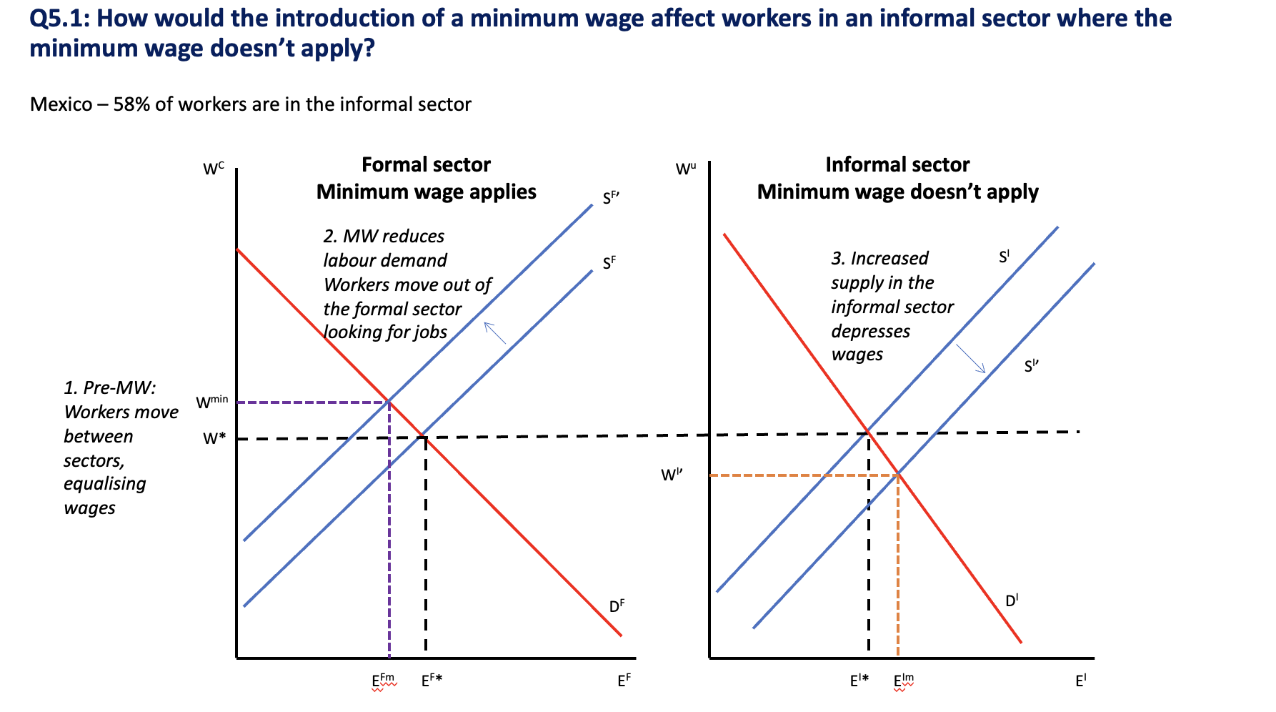
Question 5.1: How would the introduction of a minimum wage affect the employment and wages of skilled (= high wage) workers? What about workers in an informal sector where the minimum wage doesn’t apply?

Answer: within the framework of the standard model, effect on employment is ambiguous, combination of

• Substitution Effect
• Scale Effect

And the effect on wages depends on the employment effect.

Question 5.2: According to the Hicks-Marshall law of derived demand, which four factors affect the employment response to a minimum wage increase?

The size of the reduction depends on substitution and scale effects.

The papers discuss last week generally focus on a particular city/industry.

Empirical studies show little negative employment effects, Which, in this environment, means demand for low-wage labour is inelastic

• Elasticity of factor substitution (substitution effect)

Firms can’t easily substitute other factors for low-wage labour (eg fixed technology, regulations)

Putty-clay model

• Elasticity of supply of other factors (substitution effect)

Supply of capital is inelastic, making it costly to substitute

• Price elasticity of (product) demand (scale effect)

Product demand is inelastic; higher factor prices can be passed on as higher product prices

• Factor share in total costs (scale effect)

Low-wage labour is a small share of total costs; cost/ price increases are small

The drawback of the large amount of papers in the empirical papers are they only focus on the short-time effect

Competitive market for low-wage labour:

Law of one price, i.e. single, market-clearing wage rate

Wage dispersion

• Different worker-types (LOP (Law of One Price) still holds for same type?)
• Or imperfect/ monopsonistic competition in the labour market

Why some of the biggest beneficiaries are in the middle of the income distribution?

Because the MW law might not well-targeted on the poorest households.

Different Countries

US

Federal MW.

UK

An independent advisory body: Low Pay Commission (LPC).

But some countries don’t have minimum wage at all, like Italy and Austria. This makes the international comparison become very hard. One way is to use Kaitz Index

Efficiency

Minimum Wage under Imperfect Competition

结合课件内容和历年考题（2020、2021、2023、2024 均考过 MW 相关题），以下是备考重点：

---

A. 理论基础

A1. 完全竞争下的 MW 效应

• 三个关键假设：price-taking, homogeneous labour, full compliance and coverage [第 20 页]
• 核心结论：$w_{MW}>w^{\ast }$ 导致 $E_{MW}<E^{\ast }$，产生 involuntary unemployment 和 deadweight loss [第 20 页]
• 就业弹性公式：$\Delta \ln E\approx \eta \cdot \Delta \ln w$，效应 unambiguously negative [第 22 页]
• 要能画图说明 binding price floor 的效果 [第 21 页]

A2. 不完全竞争（Monopsony）下的 MW 效应

• Monopsony 条件：$MRPL=MCL$ 且 $MCL>w$（因为 upward-sloping labour supply）[第 25 页]
• 企业压低工资和就业：$w_0<w^{\ast }$ , $E_0<E^{\ast }$ [第 25 页]
• 适度 MW（$w_0<w_{MW}<w^{\ast }$）反而增加就业，因为 MW 使 MCL 在 MW 处变平 [第 25-27 页]
• 要能画图并解释 MW 如何消除 monopsony wedge [第 26 页]

A3. 两个模型的对比（“MW puzzle”）

• 竞争模型预测：higher labor cost → price increase → output demand falls → employment falls [第 87 页]
• Monopsony 预测：employment increases → firms sell more → price falls [第 87 页]
• 实证观察：positive price effects + limited employment changes，两个模型都无法完全解释 [第 87 页]

---

B. Bite 的概念与度量

• Kaitz index: ${\text{Kaitz}}_{ct}=\frac{M{W}_{ct}}{{\text{Median Wage}}_{ct}}$ [第 15 页]
• 其他度量：MW/mean wage, share of workers at or below MW, excess mass at MW [第 15 页]
• 考试高频考点：2021 年真题(c)问为什么 restaurant sector 被重点研究——因为 bite 最大；2023 年真题(a)直接考 bite 和 coverage 的概念如何应用于 racial inequality 分析

---

C. 实证方法演进（核心考试板块）

以下内容是层层递进的关系

C1. Time series（第 31 页）

• Specification: $\ln y_t=\alpha +\eta \ln (w_t)+x_t^{\prime }\delta +{\epsilon }_t$
• 结果：$\eta \in [-0.3,-0.1]$ for teens (Brown et al. 1982)
• 三个问题：OVB, measurement error, serial correlation [第 31 页]

为什么会存在 OVB 问题？

C2. State panel — Neumark & Wascher (1992)（第 33-34 页）

• Specification: $\ln y_{st}=\alpha +\eta \ln (w_{st})+x_{st}^{\prime }\delta +{\gamma }_s+{\gamma }_t+{\epsilon }_{st}$
• 识别来源：within-state MW variation，controlling for state FE and time FE [第 33 页]
• 结果：$\eta \in [-0.2,-0.1]$ [第 34 页]
• 问题：cross-state spillovers (SUTVA), differential trends, treatment effect heterogeneity [第 34 页]
• Card & Krueger (1995) “Myth and Measurement” 的三点批评：sample extension 后 MW 实际值更低、不能 reject zero、publication bias [第 35 页]

C3. Card & Krueger (1994)（考试最高频）

• 背景：1992 年 4 月 NJ MW 从 $4.25涨到$5.05，PA 不变 [第 38 页]
• DiD specification: $\Delta E_i=\eta \cdot N{J}_i+\gamma X_i+{\epsilon }_i$ [第 42 页]
• GAP exposure specification: $\Delta E_i=\tilde{\eta }\cdot GA{P}_i+\gamma X_i+{\epsilon }_i$，$GA{P}_i=N{J}_i\times \max \{\frac{W^{min}-W_{i1}}{W_{i1}},0\}$ [第 42 页]
• 两种设计识别的参数不同：DiD = market-wide response; GAP = single firm effect holding market constant [第 43 页]
• 结果：no indication MW reduced employment [第 44 页]
• 额外发现：consumer prices 上升 [第 45 页]，store openings 正但不精确 [第 46 页]
• 批评：Hamermesh (1995) anticipation + too-short horizon [第 48 页]；Neumark & Wascher (2000) measurement issues [第 48 页]

C4. DLR (2010) Border discontinuity（考试高频）

• 先复制 NW (1992) 的 TWFE，发现 employment elasticity 约 -0.176 [第 52-54 页]
• 加入 spatial heterogeneity controls 后系数接近 0 或正 [第 55 页]
• Preferred specification 用 contiguous border county-pairs：$\ln y_{ipt}=\alpha +\eta \ln (w_{it}^M)+\delta \ln (y_{it}^{TOT})+\gamma \ln (po{p}_{it})+{\varphi }_i+{\tau }_{pt}+{\epsilon }_{ipt}$ [第 57 页]
• ${\tau }_{pt}$ = pair-specific time FE，控制同一边界两侧的 common shocks [第 57 页]
• 识别假设：$E[\ln (w_{it}^M),{\epsilon }_{ipt}]=0$ [第 57 页]
• 结果：employment elasticity = 0.016，implied labour demand elasticity close to 0 and insignificant [第 59 页]
• 核心 insight：之前的负效应是由 unobserved regional differences in employment growth 导致的 downward bias [第 52 页]

C5. Cengiz et al. (2019) Bunching estimator（2021 年考题直接考）

• Specification: $\frac{E_{sjt}}{N_{st}}={\sum }_{\tau }{\sum }_k{\alpha }_{\tau k}{I}_{sjt}^{\tau k}+{\mu }_{sj}+{\rho }_{jt}+{\Omega }_{sjt}+{\upsilon }_{sjt}$ [第 69-70 页]
• $\tau$ : time relative to MW increase; $k$ : wage bin distance from new MW [第 69 页]
• FE 结构：${\mu }_{sj}$ state-by-wage-bin FE, ${\rho }_{jt}$ quarter-by-wage-bin FE [第 69 页]
• 识别假设：整个 wage distribution 在 treated 和 untreated states 之间满足 parallel trends [第 69 页]
• 核心结果：missing jobs below MW ( $\Delta b$ ) 和 excess jobs above MW ( $\Delta a$ ) 基本相等 → 总就业不变 [第 71页]
• 时间维度：missing 和 excess 在 MW 提高后同步出现并持续 [第 72 页]

C6. Manning (2021) — 总结性文献

• 工资效应 clear and positive [第 62 页]
• 就业效应 clearly not robust，对 specification 极度敏感 [第 63 页]
• Employment elasticities vary across countries and groups [第 64 页]

---

D. Beyond Employment（近年考试趋势）

D1. Incidence — Harasztosi & Lindner (2019)（第 75-84 页）

• 匈牙利 MW 涨幅极大（57% + 25%）[第 75 页]
• Specification: $\frac{y_{it}-y_{i,2000}}{y_{i,2000}}={\alpha }_t+{\beta }_{t}F{A}_i+{\gamma }_t{X}_{it}+{\epsilon }_{it}$ [第 77 页]
• $F{A}_i$ = fraction of workers for whom MW binds（连续 treatment intensity）[第 77 页]
• 就业弹性 negative but small [第 78-79 页]
• 关键发现：consumers 承担约 75%，firm owners 约 25% [第 84 页]
• 调整 margins：consumer prices 上升、labor substituted by capital [第 75 页, 82-83 页]

D2. Firm value — Bell & Machin (2018)（第 89-92 页）

• Event study: $CA{R}_{it}={\beta }_1{A}_t{D}_i+{\theta }_t{D}_i+{\delta }_t+{\epsilon }_{it}$ [第 90 页]
• $A_t$ = announcement dummy, $D_i$ = 低工资企业 dummy [第 90 页]
• 结果：low-wage firms 股价显著下跌，幅度与预期利润损失一致 [第 91-92 页]

D3. Wage inequality — Autor, Manning & Smith (2016)（第 93-97 页）

• MW 压缩 lower tail (50/10)，对 upper tail (90/50) 无影响 [第 94-95 页]
• Specification: $w_{st}(p)-w_{st}(50)=\beta (p)f([w_{st}^{min}-w_{st}(50)])+{\sigma }_s(p)+{\sigma }_s(p)\times t+{\eta }_t(p)+{\epsilon }_{st}(p)$ [第 96 页]
• $f(\cdot )$ 是 quadratic，捕捉 MW 对 more binding 的 percentile 影响更大 [第 96 页]

D4. Reallocation & productivity

• Dustmann et al. (2021)：MW 导致 low-wage workers 向 better firms 重新配置 [第 85 页]
• Coviello et al. (2022)：MW 提高后 low-type workers 生产率上升，被解雇概率下降 [第 101-102 页]
• Informal sector（巴西）：formal sector MW 在 informal sector 也 binding，但无显著的 formal → informal 重新配置 [第 99-100 页]

---

E. 考试策略提示

根据历年真题，MW 题目通常是以某篇论文为载体，考察三个层面：

1. 解读实证结果：给你图表，要求你解释 $\Delta a$ , $\Delta b$ , implied elasticity，并判断是否与 competitive model 一致（如 2021 Q4(a)(b)）
2. 方法论评价：识别假设是什么、可能的 threats、与其他方法的比较（如 DLR 对 NW 的改进）
3. 文献整合讨论：要求你结合 broader MW literature 讨论某个 finding（如 2021 Q4(d) 要求结合 Harasztosi & Lindner 等讨论 firms adjusting through different margins）