Capital Income Tax

Macro

Recall some model setting:

• Government Spending: $G=\gamma Y$
• Tax Revenue:
  • Lump-sum tax $T$ (We usually ignore it)
  • Labour-income tax ${\tau }_w$
  • Capital-income tax ${\tau }_r$ (What we are interested in this chapter)

Government Side

$$G=T+{\tau }_{r}rK+{\tau }_{w}wl$$

We are going to change ${\tau }_r$(holding $\gamma$ constant) to see how ${\tau }_r$ affects the macroeconomy.

Which means we will assume that Government Spending does not change.

Household Side

Recall, for household, we want to maximize their utility:

$$u=\ln C+\beta \ln (L-l)+v(G)$$

the maximization problem is:

$$ma{x}_{C,l}U=\sum _{t=0}\frac{\ln C_t+\beta \ln (L-l_t)+v(G_t)}{(1-\rho {)}^t}$$

s.t.

$$\dot{K}=I=wl+rK-{\tau }_{r}rK-T-C$$

It is intuitive to use the Hamiltonian to calculate the best answer, lets do this again:

$$\begin{array}{rl}\frac{\delta H}{\delta C}& =\frac{1}{C}-\lambda =0⟹\lambda =\frac{1}{C}\\ \frac{\delta H}{\delta l}& =-\frac{\beta }{L-l}+\lambda w=0⟹\lambda w=\frac{\beta }{L-l}\\ \frac{\delta H}{\delta K}& =\lambda \underset{\text{after-tax capital rental price}}{\underbrace{(1-{\tau }_{r}r)}}=\rho \lambda -\dot{\lambda }\\ ⟹-& \frac{\dot{\lambda }}{\lambda }=(1-{\tau }_r)r-\rho \end{array}$$

From the equations above, we could get:

$$\frac{\dot{C}}{C}=(1-{\tau }_r)r-\rho$$

Steady State: happens at $\dot{C}=0⟹K_{LR}^S:r=\frac{\rho }{1-{\tau }_r}$

When ${\tau }_r$ increases, the long-run capital supply curve shifts upward (i.e., reduction in supply).

When the government taxes capital income move heavily, the household accumulates less capital.

Similar, we could get from first two equations:

$$l^s:w=\frac{\beta C}{L-l}$$

Graphically Speaking:

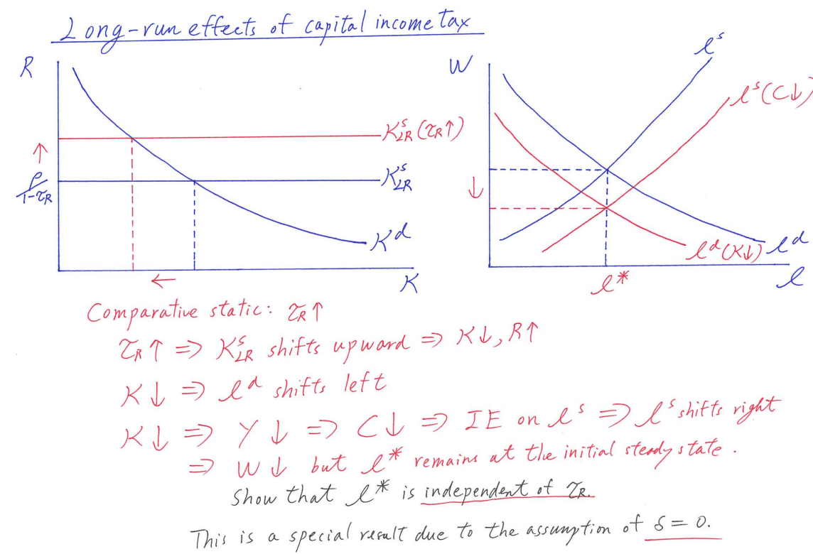
Note that the change in ${\tau }_r$ will first affect the Capital Market

To check why the $l^{\ast }$ is independent (that is to say, doesn’t change)

Deriving the steady-state level of labor $l^{\ast }$.

$$\begin{array}{rl}{l}^d:& w=MPL=\underset{\text{For Wage}}{\underbrace{(1-\alpha )A{\left(\frac{K}{l}\right)}^{\alpha }}}=\underset{\text{For Labor}}{\underbrace{(1-\alpha )U\frac{Y}{l}}}\\ l^s:& w=\frac{\beta C}{L-l}⟹l^s=L-\frac{\beta C}{w}\\ l^s& =l^d:l=L-\frac{\beta C}{(1-\alpha )Y}l\end{array}$$

Finally, we could get:

$$l=\frac{L}{1+\frac{\beta }{1-\alpha }\frac{C}{Y}}$$

Given that $\delta =0$, $\frac{C}{Y}=1-\gamma$

$$l^{\ast }=\frac{L}{1+\frac{\beta }{1-\alpha }(1-\gamma )}$$

is independent of ${\tau }_w$

Deriving the Consumption-output ratio

$$\dot{K}=I=wl+rK-({\tau }_{r}rK+T)-C$$ $$⟹Y-\gamma Y-C$$

At steady state: $\dot{K}=0⟹C=(1-\gamma )Y$

In the output market: $Y=A{K}^{\alpha }{l}^{(1-\alpha )}$

$${\tau }_r\uparrow ⟹K\downarrow ⟹Y\downarrow ⟹C\downarrow$$

Exercise

1. Derive $l^{\ast }$ when $\delta >0$, show that $l^{\ast }$ depends on ${\tau }_r$ if $\delta >0$

Answer: recall the definition of $\delta$ is the capital depreciation rate,

Now, the asset-accumulation equation of $\dot{K}$ becomes:

$$\begin{array}{rl}\dot{K}& =I=wl+rK-{\tau }_{r}rK-T-C-\delta K\\ & =[r-{\tau }_{r}r-\delta ]K+wl-C-T\end{array}$$

We should then redo the Hamiltonian:

$$\begin{array}{rl}\frac{\delta H}{\delta C}& =\frac{1}{C}-\lambda =0⟹\lambda =\frac{1}{C}\\ \frac{\delta H}{\delta l}& =-\frac{\beta }{L-l}+\lambda w=0⟹\lambda w=\frac{\beta }{L-l}\\ \frac{\delta H}{\delta K}& =\lambda (r-{\tau }_{r}r-\delta )=\rho \lambda -\dot{\lambda }\\ ⟹-& \frac{\dot{\lambda }}{\lambda }=(1-{\tau }_r)r-\delta -\rho \end{array}$$

Use the 1, 3 equation:

We could get:

$$\frac{\dot{C}}{C}=(1-{\tau }_r)r-\delta -\rho$$

Also recall the equation we use when finding the $l^{\ast }$:

$$l^s=l^d:l=L-\frac{\beta C}{(1-\alpha )Y}l$$

Since it is at the steady state, that is $\dot{C}=0$,

$$\begin{array}{rl}\dot{K}& =I=\underset{Y}{\underbrace{wl+rK}}-\underset{G=\gamma Y}{\underbrace{{\tau }_{r}rK+T}}-C-\delta K=0\\ 0& =Y-{\tau }_{r}rK-C-\delta K\\ C& =Y-{\tau }_{r}rK-\delta K\\ \frac{C}{Y}& =(1-\gamma )\frac{Y}{Y}-\frac{\delta K}{Y}\end{array}$$

That is to say, we have to derive $\frac{K}{Y}$

At long-run,

$$\begin{array}{rlr}{K}^d:& r=\alpha \frac{Y}{K}⟹\frac{K}{Y}=\frac{\alpha }{r}& \\ K^s:& \dot{C}=0⟹(1-{\tau }_r)r=\rho +\delta ⟹r=\frac{\rho +\delta }{1-{\tau }_r}& \end{array}$$

So that when $K^d=K^s$, we could get: $\frac{K}{Y}=\frac{\alpha (1-{\tau }_r)}{(\rho +\delta ))}$

That is, $\frac{C}{Y}=(1-\gamma )-\frac{\delta \alpha (1-{\tau }_r)}{\rho +\delta }$

So we plug it in the original equation, the we could get:

$$l^{\ast }=\frac{L}{1+\frac{\beta }{1-\alpha }[(1-\gamma )-\frac{\delta \alpha (1-{\tau }_r)}{\rho +\delta }]}$$

Exercise for Capital Income Tax

Capital Taxation in the Neoclassical Growth Model

Household

$$ma{x}_{C,l}U=\sum _{t=0}\frac{\ln C_t+\beta \ln (L-l_t)+v(G_t)}{(1-\rho {)}^t}$$

s.t.

$$\dot{K}=I-\delta K=wl+rK-{\tau }_{r}rK-T-C-\delta K$$

Then we redo the Hamiltonian, but the steps are the as what we see in Exercise for Capital Income Tax